 |
 |
 |
 | A robust approach to time-to-depth conversion and interval velocity
estimation from time migration in the presence of lateral velocity variations |  |
![[pdf]](icons/pdf.png) |
Next: Bibliography
Up: Li & Fomel: Time-to-depth
Previous: Appendix C: Analytical expressions
In this appendix, we study the following medium:
 |
(55) |
where
![$\mathbf{q} = [0,q_x]^T$](img197.png) .
.
Similarly to the constant velocity gradient medium, it is convenient to write down the ray-tracing system in
the form (Cervený, 2001)
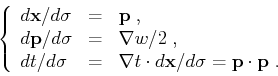 |
(56) |
Given equation D-1,
 and thus
 .
After integration over
.
After integration over  , equation D-2 becomes
 |
(57) |
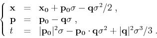
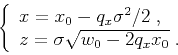
For a particular image ray
![\begin{displaymath}
\left\{ \begin{array}{lcl}
\mathbf{x_0} & = & [0, x_0]^T\;, ...
...0 - 2 q_x x_0}, 0]^T\;, \\
t_0 & = & t\;,
\end{array} \right.
\end{displaymath}](img203.png) |
(58) |
the equation for  in D-3 simplifies to
 |
(59) |
Solving equation D-5 for as a function of  and
and 
![\begin{displaymath}
\sigma (z,x) = \left[ \frac{(w_0 - 2 q_x x)
- \sqrt{(w_0 - 2 q_x x)^2 - 4 q_x^2 z^2}}{2 q_x^2}
\right]^{\frac{1}{2}}\;.
\end{displaymath}](img205.png) |
(60) |
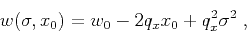
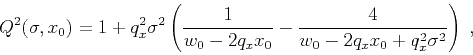
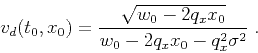
Combining equations D-3 through D-6, we find
According to equation 4, D-7 can give rise to the geometrical spreading:
![\begin{displaymath}
Q^2 (z,x) =
\frac{2 [(w_0 - 2 q_x x)^2 - 4 q_x^2 z^2]}
{(w_0...
...- 2 q_x x + \sqrt{(w_0 - 2 q_x x)^2 - 4 q_x^2 z^2} \right]}\;.
\end{displaymath}](img212.png) |
(63) |
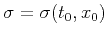
It is more convenient to express equations D-1 and D-9 in and  instead
of directly in
instead
of directly in  and :
and :
 |
(64) |
 |
(65) |
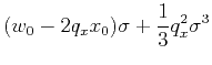
where we must resolve
 . This is done by revisiting equation D-8. For
given and , is the root of a depressed cubic function of the following form:
. This is done by revisiting equation D-8. For
given and , is the root of a depressed cubic function of the following form:
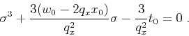 |
(66) |
After some algebraic manipulations, we find
Finally, inserting equations D-10 and D-11 into equation 3 results
in the Dix velocity:
 |
(68) |
|
|
|
|
| A robust approach to time-to-depth conversion and interval velocity
estimation from time migration in the presence of lateral velocity variations | |
|
Next: Bibliography
Up: Li & Fomel: Time-to-depth
Previous: Appendix C: Analytical expressions
2015-03-25

![$\displaystyle \frac{\sqrt{2} z \left[ 2 w_0 - 4 q_x x + \sqrt{(w_0 - 2 q_x x)^2...
..._0 - 2 q_x x + \sqrt{(w_0 - 2 q_x x)^2 - 4 q_x^2 z^2} \right]^{\frac{1}{2}}}\;.$](img211.png)
![$\displaystyle \left[ \frac{3 t_0 + \sqrt{9 t_0^2 + 4 (w_0 - 2 q_x x_0)^3 / q_x^2}}{2 q_x^2} \right]^{\frac{1}{3}}$](img218.png)
![$\displaystyle \frac{w_0 - 2 q_x x_0}{q_x}
\left[ \frac{2}{3 q_x t_0 + \sqrt{9 q_x^2 t_0^2 + 4 (w_0 - 2 q_x x_0)^3}} \right]^{\frac{1}{3}}\;.$](img220.png)