|
|
|
|
Missing log data interpolation and semiautomatic seismic well ties using data matching techniques |
Next: Seismic-well tie example Up: Missing log data estimation Previous: Teapot Dome Well Log
|
|
|
|
Missing log data interpolation and semiautomatic seismic well ties using data matching techniques |
Synthetic seismograms are modeled independently for each well. White and Simm (2003) argue that modeling synthetic seismograms benefits from blocking or upscaling of the logs. Following their suggestion, we upscale the sonic and density logs to seismic frequencies (Backus, 1962; Marion et al., 1994) and estimate an initial reflectivity series, ![]() , in depth assuming no multiples, attenuation or dispersion.
, in depth assuming no multiples, attenuation or dispersion.
The initial TDR relates the initial reflectivity series, ![]() , to time. We interpolate the resulting reflectivity series in time to a regularly sampled grid of 0.002s, which corresponds to the vertical sampling of the seismic data.
, to time. We interpolate the resulting reflectivity series in time to a regularly sampled grid of 0.002s, which corresponds to the vertical sampling of the seismic data.
We model synthetic seismograms by convolving ![]() with a single, zero-phase, wavelet that is representative of the seismic data's frequency content. The zero-phase wavelet extracted using Hampson Russell software is shown in Figure 13.
with a single, zero-phase, wavelet that is representative of the seismic data's frequency content. The zero-phase wavelet extracted using Hampson Russell software is shown in Figure 13.

|
|---|
|
wavelet200
Figure 13. Statistical wavelet extracted from the Teapot Dome seismic dataset. |
|
|
Using the statistical wavelet in Figure 13 and the initial TDR, we compute a synthetic seismogram shown in Figure 14 (green). We then iteratively estimate the alignment shifts, ![]() , by using the LSIM method to match the synthetic seismogram (red) to the corresponding real seismic trace in Figure 14 (black).
, by using the LSIM method to match the synthetic seismogram (red) to the corresponding real seismic trace in Figure 14 (black).
In the time domain, the shifts,
![]() at well
at well ![]() , are estimated using several iterations,
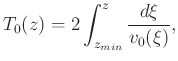
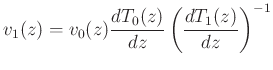
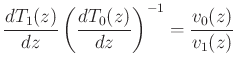
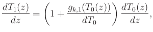
, are estimated using several iterations, ![]() , of LSIM data matching. Each iteration estimates a smooth sequence of shifts to align the synthetic seismogram with the seismic trace. Muñoz and Hale (2015) and Herrera et al. (2014) observe a relationship between the shifts used to align a synthetic with seismic trace and an updated velocity function:
, of LSIM data matching. Each iteration estimates a smooth sequence of shifts to align the synthetic seismogram with the seismic trace. Muñoz and Hale (2015) and Herrera et al. (2014) observe a relationship between the shifts used to align a synthetic with seismic trace and an updated velocity function:
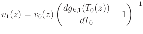
From Equation 2, assuming an initial TDR, ![]() , we arrive at updated estimate
, we arrive at updated estimate
 |
(14) |
 |
(16) |
 |
(17) |
We update the velocity function and recompute Equations 9, 10, and 11 after each iteration of estimating shifts using LSIM. We slowly reduce the smoothness enforced by regularization in LSIM with each iteration to ensure that stretching and squeezing are not excessive thus resulting in an improbable velocity update (White and Simm, 2003).
Prior to performing the seismic-well tie, we need to understand phase variations and distortions introduced during the processing and imaging of the seismic data. There are several seismic processing and imaging techniques that adjust or correct the seismic data to zero phase. Information on phase adjustments applied to the data are not available; however, Harbert (2012) interprets the deepest continuous reflection to be Precambrian basement resulting in a positive amplitude![]() . As provided by the U.S. Department of Energy and RMOTC, the basement reflection is a negative amplitude. To account for the observed lateral and vertical phase variations, we apply local skewness correction (Fomel and van der Baan, 2014) resulting in a zero-phased seismic volume consistent with observations from Harbert (2012).
. As provided by the U.S. Department of Energy and RMOTC, the basement reflection is a negative amplitude. To account for the observed lateral and vertical phase variations, we apply local skewness correction (Fomel and van der Baan, 2014) resulting in a zero-phased seismic volume consistent with observations from Harbert (2012).
|
|
|
|
Missing log data interpolation and semiautomatic seismic well ties using data matching techniques |