|
|
|
|
Simulating propagation of separated wave modes in general anisotropic media, Part I: qP-wave propagators |
For comparison, we first appply the original anisotropic elastic wave equation
to synthesize wavefields in a homogeneous VTI medium with weak anisotropy, in which
![]() ,
,
![]() ,
,
![]() , and
, and
![]() .
Figure 4a and 4b display the horizontal and vertical components of the displacement wavefields at 0.3 s.
Then we try to simulate propagation of separated wave modes using the pseudo-pure-mode qP-wave equation
(equation 22 in its 2D form).
Figure 4c and 4d display the two components of the pseudo-pure-mode qP-wave fields, and Figure 4e
displays their summation, i.e., the pseudo-pure-mode scalar qP-wave fields with weak residual qSV-wave energy.
Compared with the theoretical wavefront curves (see Figure 4f) calculated
on the base of group velocities
and angles, pseudo-pure-mode scalar qP-wave fields have correct kinematics for both qP- and qSV-waves.
We finally remove residual qSV-waves and get completely separated scalar qP-wave fields by
applying the filtering to correct the projection deviation (Figure 4g).
.
Figure 4a and 4b display the horizontal and vertical components of the displacement wavefields at 0.3 s.
Then we try to simulate propagation of separated wave modes using the pseudo-pure-mode qP-wave equation
(equation 22 in its 2D form).
Figure 4c and 4d display the two components of the pseudo-pure-mode qP-wave fields, and Figure 4e
displays their summation, i.e., the pseudo-pure-mode scalar qP-wave fields with weak residual qSV-wave energy.
Compared with the theoretical wavefront curves (see Figure 4f) calculated
on the base of group velocities
and angles, pseudo-pure-mode scalar qP-wave fields have correct kinematics for both qP- and qSV-waves.
We finally remove residual qSV-waves and get completely separated scalar qP-wave fields by
applying the filtering to correct the projection deviation (Figure 4g).


|
|---|
|
Elasticx,Elasticz,PseudoPurePx,PseudoPurePz,PseudoPureP,WF,PseudoPureSepP
Figure 4. Synthesized wavefields in a VTI medium with weak anisotropy: (a) x- and (b) z-components synthesized by original elastic wave equation; (c) x- and (d) z-components synthesized by pseudo-pure-mode qP-wave equation; (e) pseudo-pure-mode scalar qP-wave fields; (f) kinematics of qP- and qSV-waves; and (g) separated scalar qP-wave fields. |
|
|
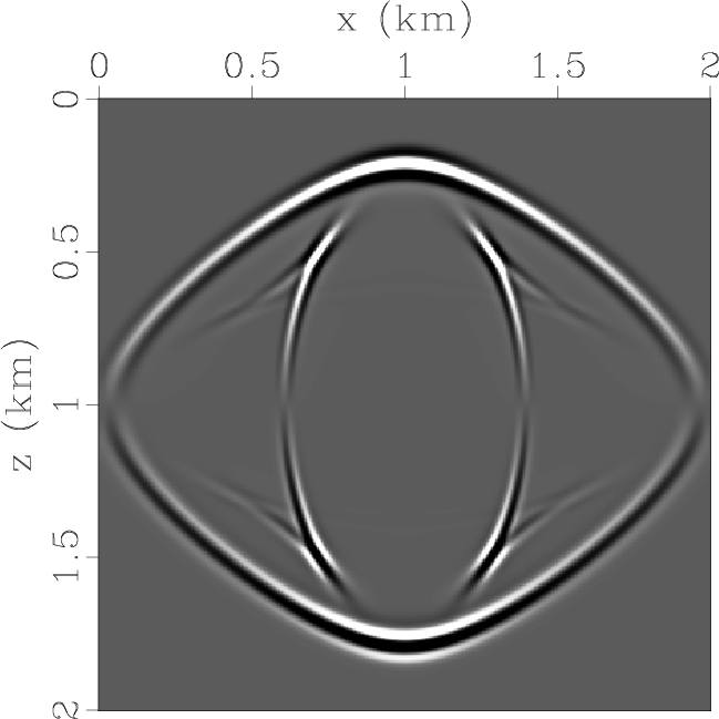
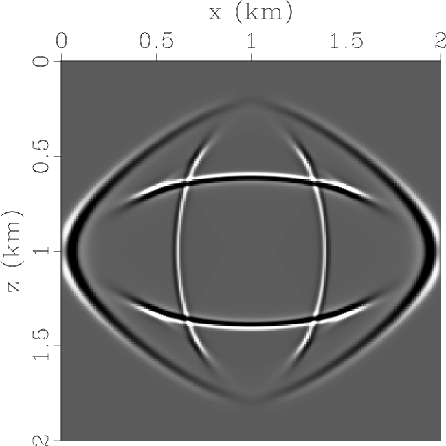
Then we consider wavefield modeling in a homogeneous VTI medium with strong anisotropy,
in which
![]() ,
,
![]() ,
,
![]() , and
, and
![]() .
Figure 5 displays the wavefield snapshots at 0.3 s synthesized by using original elastic wave equation
and pseudo-pure-mode qP-wave equation respectively. Note that the pseudo-pure-mode qP-wave fields still accurately
represent the qP- and qSV-waves' kinematics. Although the residual qSV-wave energy becomes stronger when
the strength of anisotropy increases, the filtering step still removes these residual qSV-waves effectively.
.
Figure 5 displays the wavefield snapshots at 0.3 s synthesized by using original elastic wave equation
and pseudo-pure-mode qP-wave equation respectively. Note that the pseudo-pure-mode qP-wave fields still accurately
represent the qP- and qSV-waves' kinematics. Although the residual qSV-wave energy becomes stronger when
the strength of anisotropy increases, the filtering step still removes these residual qSV-waves effectively.


|
|---|
|
Elasticx,Elasticz,PseudoPurePx,PseudoPurePz,PseudoPureP,WF,PseudoPureSepP
Figure 5. Synthesized wavefields in a VTI medium with strong anisotropy: (a) x- and (b) z-components synthesized by original elastic wave equation; (c) x- and (d) z-components synthesized by pseudo-pure-mode qP-wave equation; (e) pseudo-pure-mode scalar qP-wave fields; (f) kinematics of qP- and qSV-waves; and (g) separated scalar qP-wave fields. |
|
|
|
|
|
|
Simulating propagation of separated wave modes in general anisotropic media, Part I: qP-wave propagators |