|
|
|
|
Simulating propagation of separated wave modes in general anisotropic media, Part II: qS-wave propagators |
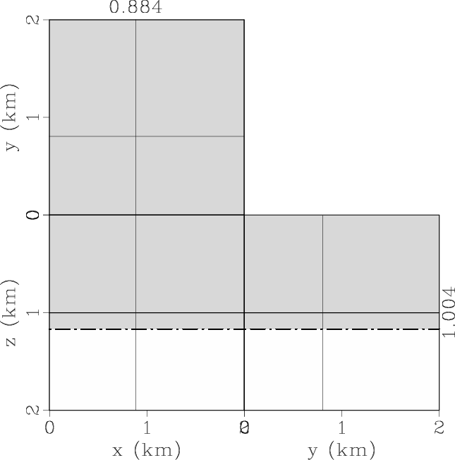
Figure 4 shows an example of simulating the propagation of pseudo-pure-mode qSV-wave fields in a 3D two-layer
VTI model (see Figure 4a), with
![]() ,
,
![]() ,
,
![]() ,
,
![]() and
and
![]() in the first layer, and
in the first layer, and
![]() ,
,
![]() ,
,
![]() ,
,
![]() and
and
![]() in the second layer.
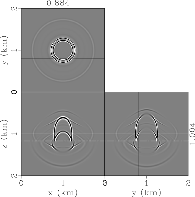
We propagate the 3D pseudo-pure-mode qSV-wave fields using equation 28.
Figure 4d displays the pseudo-pure-mode scalar qSV-wave fields resulting from the summation of
the horizontal (Figure 4b) and vertical (Figure 4c) components, namely
in the second layer.
We propagate the 3D pseudo-pure-mode qSV-wave fields using equation 28.
Figure 4d displays the pseudo-pure-mode scalar qSV-wave fields resulting from the summation of
the horizontal (Figure 4b) and vertical (Figure 4c) components, namely
![]() and
and
![]() .
We see that the qS-waves dominate the scalar wavefields in energy.
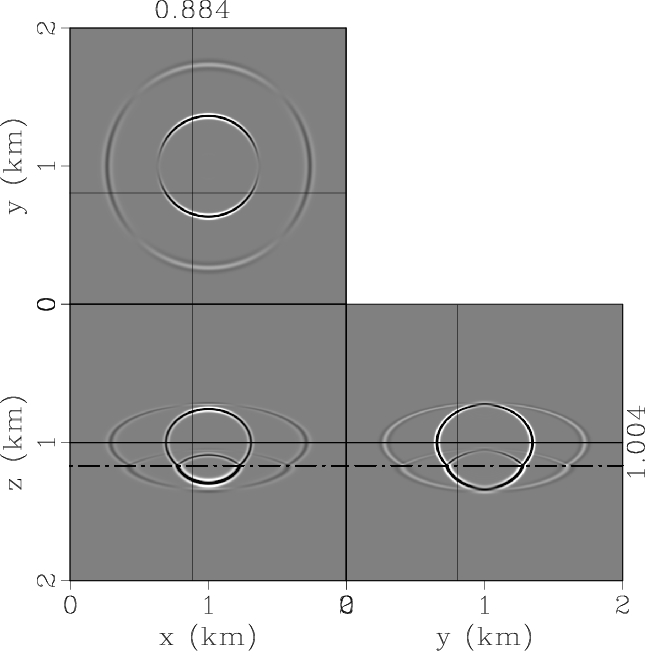
As shown in Figure 5, we also obtain pure-mode scalar SH-wave fields either using the summation of the horizontal components
synthesized by using the pseudo-pure-mode wave equation 17 or directly using the scalar wave equation, i.e., equation 18.
.
We see that the qS-waves dominate the scalar wavefields in energy.
As shown in Figure 5, we also obtain pure-mode scalar SH-wave fields either using the summation of the horizontal components
synthesized by using the pseudo-pure-mode wave equation 17 or directly using the scalar wave equation, i.e., equation 18.


|
|---|
|
vp0Interf,PseudoPureSVxyInterf,PseudoPureSVzInterf,PseudoPureSVInterf
Figure 4. Synthesized wavefield snapshots in a 3D two-layer VTI model using equation 28 : (a) vertical velocity of qSV-wave, (b) horizontal component |
|
|


|
|---|
|
SHxInterf,SHyInterf,SHInterf
Figure 5. Synthesized wavefield snapshots in a 3D two-layer VTI model using equation 17: (a) x- and (b) y-components of the pseudo-pure-mode wavefields, (c) pure-mode scalar SH-wave fields calculated as the summation of the two horizontal components of the pseudo-pure-mode wavefields. Note that the same scalar wavefields are obtained if we directly use the scalar wave equation for SH-waves, namely equation 18. |
|
|
|
|
|
|
Simulating propagation of separated wave modes in general anisotropic media, Part II: qS-wave propagators |