|
|
|
|
IWAVE Structure and Basic Use Cases |

|
|---|
|
gauss
Figure 2. Gaussian initial datum |
|
|
The data depicted in Figures 1 and 2 is input to the simulation, so clearly must exist prior to simulation. However the output must also exist: IWAVE I/O, both reads and writes, is driven by the target data structure. Therefore the movie output file must be constructed before the simulation fills it with data. The SConstruct script contains an invocation of the sfmakevel command which creates a 3D rsf file movieinit.rsf. On completion of the command, this file holds the movie output.
Perusal of this command reveals some customization of the rsf file format, as compared to its standard use (Fomel et al. (2013)). The duration of the movie determines the duration of the simulation: the initial simulation time is the time of the initial movie frame, and similarly for the final time. Thus IWAVE must be able to determine which axis specified in movieinit.rsf is the time axis. Three additional header word categories, beyond those of the rsf standard, make this feat possible:
In this example, the space dimension is 2, so id3=2 indicates that the 3rd axis is the time axis.
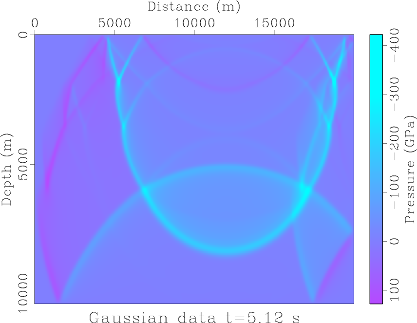
After propagating 5.12 s and interacting with both the reflecting (Dirichlet) boundaries and the interfaces in the model, the potential field becomes that depicted in Figure 3.
|
|---|
|
frameinit
Figure 3. Acoustic potential field at 5.12 s, resulting from Gaussian initial data |
|
|
Parameters passed to the command acd.x included
           csq = ../csq_4layer.rsf
         initc = ../init.rsf
         movie = ../movieinit.rsf
Keywords data and source were ignored. Many other
paramters were required; a brief description of these is included in
the self-doc of the command acd.x.
Note that the pathnames refer to the directory level above the working directory. IWAVE produces various diagnostic output at runtime, switched by various flags passed as parameters. These outputs, and possibly other auxiliary outputs of commands built upon IWAVE (eg. the data residual in an inversion) vary with application and data, so are inconvenient to specify individually as cleanup targets. Instead, the SConstruct script creates a working subdirectory and executes (and dumps its auxiliary output) there. The entire directory is cleaned up by scons -c. So the correct parameter specification for archival input and output files is one directory level up.
|
|
|
|
IWAVE Structure and Basic Use Cases |