We propose to use AB semblance by Fomel (2009) for NMO velocity analysis to handle the AVO anomalies, especially in the data that show class II polarity reversal. Conventional semblance can be interpreted as a squared correlation coefficient of seismic data with a constant while AB semblance can be considered a squared correlation coefficient with a trend (Fomel, 2009).
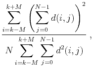
Equations 1 and 2 show the
calculation of conventional semblance (Neidell and Taner, 1971)
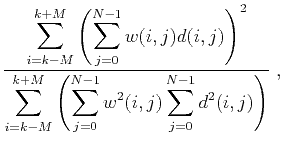
and weighted semblance (Chen et al., 2015), respectively.
AB semblance is a special case of weighted semblance; that is, substituting the weighting function
in equation 2 with a trend function
, where
is a known function related to the subsurface reflection angle or the
surface offset. Here I choose surface offset for easy calculation.
(1)
(2)
where
is the weighting function,
is the center of the
time window,
is the length of the time window,
is
the number of traces in one CMP gather,
is the
th
sample amplitude of the
th trace in the NMO-corrected
CMP gather. Appendix A gives a brief review of calculating
and
from the CMP gathers by least-squares fitting.
Weighted stacking of seismic AVO data
using hybrid AB semblance and local similarity