 |
 |
 |
 | RTM using effective boundary saving: A staggered grid GPU implementation |  |
![[pdf]](icons/pdf.png) |
Next: Effective boundary saving
Up: Yang et al.: Boundary
Previous: Introduction
In the case of constant density, the acoustic wave equation is written as
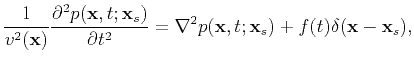 |
(1) |
where
 is the wavefield excited by the source at the position
 ,
,
 stands for the velocity in the media,
 ,
,  denotes the source signature. For the convenience, we eliminate the source term hereafter and use the notation
 and
and
 ,
,  . The forward marching step can be specified after discretization as
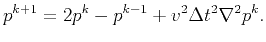 |
(2) |
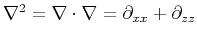
Based on the wave equation, the principle of RTM imaging can be interpreted as the cross-correlation of two wavefields at the same time level, one computed by forward time recursion, the other computed by backward time stepping (Symes, 2007).
Mathematically, the cross-correlation imaging condition can be expressed as
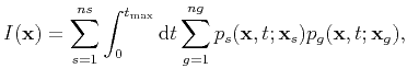 |
(3) |
where
 is the migrated image at point
  ; and
; and
 and
and
 are the source wavefield and receiver (or geophone) wavefield. The normalized cross-correlation imaging condition is designed by incorporating illumination compensation:
 |
(4) |
There are some possible ways to do RTM computation. The simplest one may be just storing the forward modeled wavefields on the disk, and reading them for imaging condition in the backward propagation steps. This approach requires frequent disk I/O and has been replaced by wavefield reconstruction method. The so-called wavefield reconstruction method is a way to recover the wavefield via backward reconstructing or forward remodeling, using the saved wavefield snaps and boundaries. It is of special value for GPU computing because saving the data in device variables eliminates data transfer between CPU and GPU. By saving the last two wavefield snaps and the boundaries, one can reconstruct the wavefield of every time step, in time-reversal order. The checkpointing technique becomes very useful to further reduce the storage (Dussaud et al., 2008; Symes, 2007). Of course, it is also possible to avert the issue of boundary saving by applying the random boundary condition, which may bring some noises in the migrated image (Liu et al., 2013b; Clapp, 2009; Liu et al., 2013a; Clapp et al., 2010).
|
|
|
|
| RTM using effective boundary saving: A staggered grid GPU implementation | |
|
Next: Effective boundary saving
Up: Yang et al.: Boundary
Previous: Introduction
2021-08-31