|
|
|
|
RTM using effective boundary saving: A staggered grid GPU implementation |
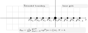
Assume ![]() -th order finite difference scheme is applied. The Laplacian operator is specified by
-th order finite difference scheme is applied. The Laplacian operator is specified by
![\begin{displaymath}\begin{array}{rl} \nabla^2 p^{k}&=\partial_{xx}p^{k}+\partial...
...frac{1}{\Delta x^2}\sum_{i=-N}^Nc_i p^k[ix+i][iz]\\ \end{array}\end{displaymath}](img65.png) |
(6) |
Keep in mind that we only need to guarantee the correctness of the wavefield in the original model zone
![]() . However, the saved wavefield in
. However, the saved wavefield in
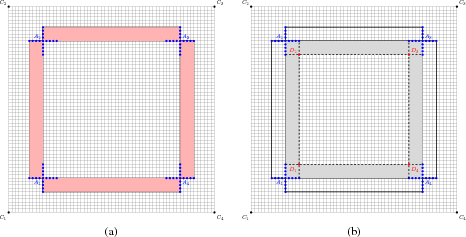
![]() is also correct. Is it possible to further shrink it to reduce number of points for saving? The answer is true. Our solution is: saving the inner
is also correct. Is it possible to further shrink it to reduce number of points for saving? The answer is true. Our solution is: saving the inner ![]() layers on each side neighboring the boundary
layers on each side neighboring the boundary
![]() , as shown in Figure 3b. We call it the effective boundary for regular finite difference scheme.
, as shown in Figure 3b. We call it the effective boundary for regular finite difference scheme.
After ![]() steps of forward modeling, we begin our backward propagation with the last 2 wavefield snap
steps of forward modeling, we begin our backward propagation with the last 2 wavefield snap ![]() and
and ![]() and saved effective boundaries in
and saved effective boundaries in
![]() . At that moment, the wavefield is correct for every grid point. (Of course, the correctness of the wavefield in
. At that moment, the wavefield is correct for every grid point. (Of course, the correctness of the wavefield in
![]() is guaranteed.) At time
is guaranteed.) At time ![]() , we assume the wavefield in
, we assume the wavefield in
![]() is correct. One step of backward propagation means
is correct. One step of backward propagation means
![]() is shrunk to
is shrunk to
![]() . In other words, the wavefield in
. In other words, the wavefield in
![]() is correctly reconstructed. Then we load the saved effective boundary of time
is correctly reconstructed. Then we load the saved effective boundary of time ![]() to overwrite the area
to overwrite the area
![]() . Again, all points of the wavefield in
. Again, all points of the wavefield in
![]() are correct. We repeat this overwriting and computing process from one time step to another (
are correct. We repeat this overwriting and computing process from one time step to another (
![]() ), in reverse time order. The wavefield in the boundary
), in reverse time order. The wavefield in the boundary
![]() may be incorrect because the points here are neither saved nor correctly reconstructed from the previous step.
may be incorrect because the points here are neither saved nor correctly reconstructed from the previous step.
|
|---|
|
fig2
Figure 2. 1-D schematic plot of required points in regular grid for boundary saving. Computing the laplacian needs |
|
|
|
|---|
|
fig3
Figure 3. A 2-D sketch of required points for boundary saving for regular grid finite difference: (a) The scheme proposed by Dussaud et al. (2008) (red zone). (b) Proposed effective boundary saving scheme (gray zone). |
|
|
|
|
|
|
RTM using effective boundary saving: A staggered grid GPU implementation |