 |
 |
 |
 | RTM using effective boundary saving: A staggered grid GPU implementation |  |
![[pdf]](icons/pdf.png) |
Next: GPU implementation using CPML
Up: Effective boundary saving
Previous: Effective boundary for staggered
For the convenience of complexity analysis, we define the size of the original model as
 . In each direction, we pad the model with the
  points on both sides as the boundary. Thus, the extended model size becomes
 . Conventionally one has to save the whole wavefield within the model size on the disk. The required number of points is
 |
(9) |
According to Dussaud et al. (2008), for  -th order finite difference in regular grid,
  points on each side are added to guarantee the correctness of inner wavefield. The saving amount of every time step is
 |
(10) |
In the proposed effective boundary saving strategy, the number becomes
 |
(11) |
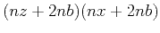
In the case of staggered grid, there are  points on each side. Allowing for four corners, the number for the effective boundary saving is
 |
(12) |
Assume the forward modeling is performed  steps using the floating point format on the computer. The saving amount will be multiplied by
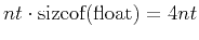 . Table 3 lists this memory requirement for different boundary saving strategies.
Table 3:
Storage requirement for different saving strategy
| Boundary saving scheme |
Saving amount (Unit: Bytes) |
| Conventional saving strategy |
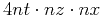
|
| Dussaud's: regular grid |
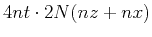
|
| Effective boundary: regular grid |
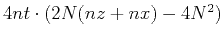
|
| Effective boundary: staggered grid |
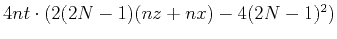
|
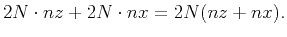
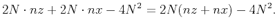
In principle, the proposed effective boundary saving will reduce
 bytes for regular grid finite difference, compared with the method of Dussaud et al. (2008). The storage requirement of staggered grid based effective boundary saving is about
  times of that in the regular grid finite difference, by observing
 . For the convenience of practical implementation, the four corners can be saved twice so that the saving burden of the effective boundary saving has no difference with the method of Dussaud et al. (2008) in regular grid finite difference. Since the saving burden for staggered grid finite difference has not been touched in Dussaud et al. (2008), it is still of special value to minimize its storage requirement for GPU computing.
|
|
|
|
| RTM using effective boundary saving: A staggered grid GPU implementation | |
|
Next: GPU implementation using CPML
Up: Effective boundary saving
Previous: Effective boundary for staggered
2021-08-31