|
 |
 |
 | A numerical tour of wave propagation |  |
![[pdf]](icons/pdf.png) |
Next: Discretization of SPML
Up: Discretization
Previous: Discretization
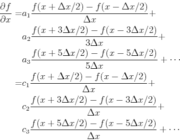
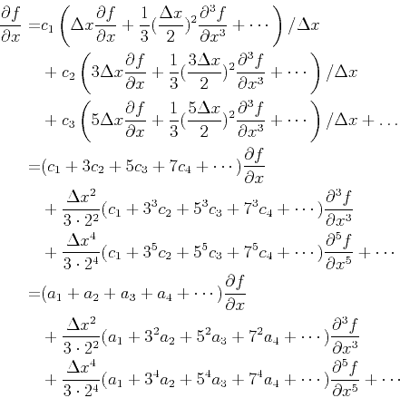
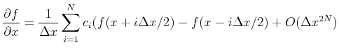
To approximate the 1st-order derivatives as accurate as possible, we express it in the following
 |
(32) |
where
 . Substituting the
  and
and  with (29) for
 results in
 |
(33) |
Thus, taking first  terms means
 |
(34) |
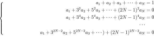
In matrix form,
 |
(35) |
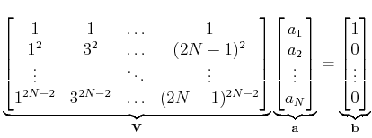
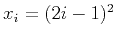
The above matrix equation is Vandermonde-like system:
 ,
,
 . The Vandermonde matrix
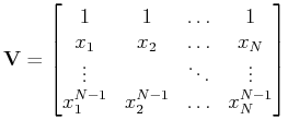 |
(36) |
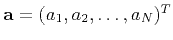
in which
 , has analytic solutions.
can be solved using the specific algorithms, see Bjorck (1996). And we obtain
, has analytic solutions.
can be solved using the specific algorithms, see Bjorck (1996). And we obtain
 |
(37) |
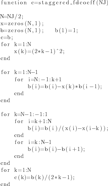
The MATLAB code for solving the 2N-order finite difference coefficients is provided in the following.
In general, the stability of staggered-grid difference requires that
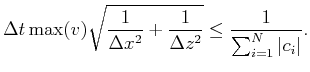 |
(38) |
Define
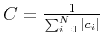 . Then, we have
In the 2nd-order case, numerical dispersion is limited when
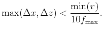 |
(39) |
The 4th-order dispersion relation is:
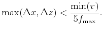 |
(40) |
|
|
|
|
| A numerical tour of wave propagation | |
|
Next: Discretization of SPML
Up: Discretization
Previous: Discretization
2021-08-31