 |
 |
 |
 | A numerical tour of wave propagation |  |
![[pdf]](icons/pdf.png) |
Next: Computation strategies and boundary
Up: Reverse time migration (RTM)
Previous: RTM implementation
Imaging condition
The cross-correlation imaging condition can be expressed as
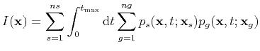 |
(55) |
where
 is the migration image value at point
  ; and
; and
 and
and
 are the forward and reverse-time wavefields at point
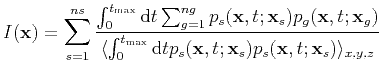
. With illumination compensation, the cross-correlation imaging condition is given by
are the forward and reverse-time wavefields at point
. With illumination compensation, the cross-correlation imaging condition is given by
 |
(56) |
in which  is chosen small to avoid being divided by zeros.
There exists a better way to carry out the illumination compensation, as suggested by Guitton et al. (2007)
 |
(57) |
where
 stands for smoothing in the image space in the x, y, and z directions.
Yoon et al. (2003) define the seismic Poynting vector as
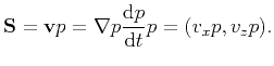 |
(58) |
Here, we denote  and
and  as the source wavefield and receiver wavefield Poynting vector. As mentioned before, boundary saving with split PML is a good scheme for the computation of Poynting vector, because
  and
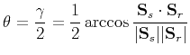
and  are available when backward reconstructing the source wavefield. The angle between the incident wave and the reflected wave can then be obtained:
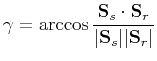 |
(59) |
The incident angle (or reflective angle) is half of  , namely,
 |
(60) |
Using Poynting vector to confine the spurious artefacts, Yoon and Marfurt (2006) propose a hard thresholding scheme to weight the imaging condition:
|
(61) |
where
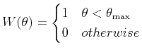 |
(62) |
Costa et al. (2009) modified the weight as
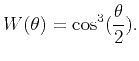 |
(63) |
These approaches are better for eliminating the backward scattering waves in image.
|
|
|
|
| A numerical tour of wave propagation | |
|
Next: Computation strategies and boundary
Up: Reverse time migration (RTM)
Previous: RTM implementation
2021-08-31