A numerical tour of wave propagation

Numerical examples

I show my GPU-based RTM result for two benchmark models: Marmousi model (Versteeg, 1994) and Sigsbee model (DiMarco et al., 2001). Here, I use CPML boundary condition to obtain high quality imaging result.

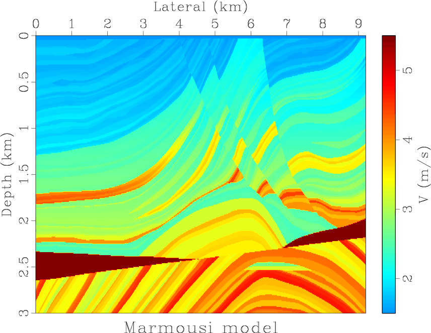
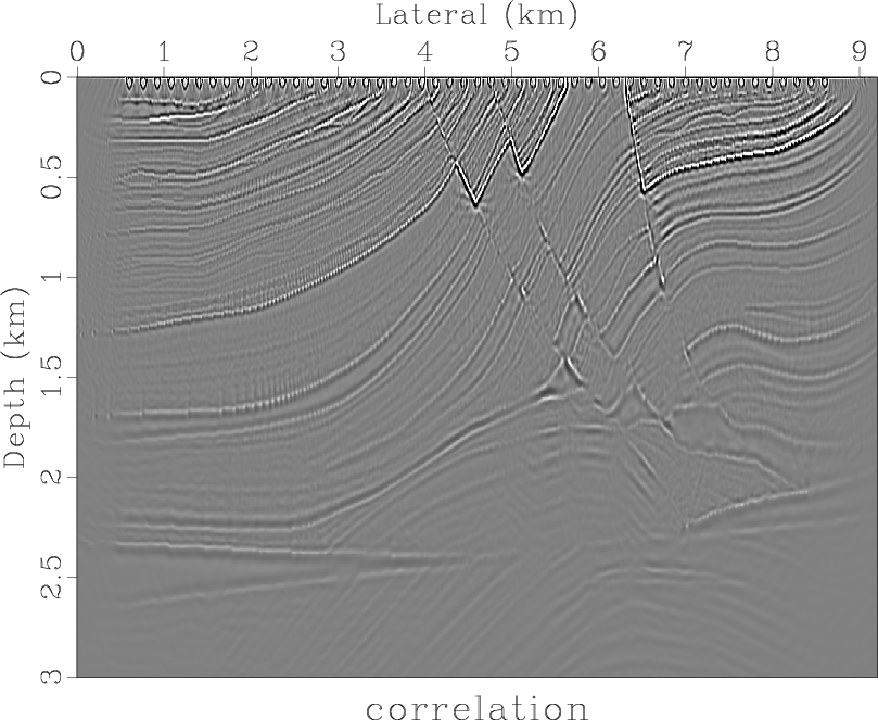
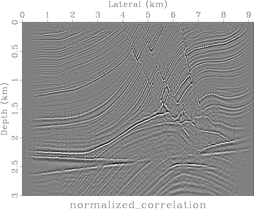
The Marmousi model is shown in Figure 11. The spatial sampling interval is $\Delta x=\Delta z=4m$ . 51 shots are deployed. In each shot, 301 receivers are placed in the split shooting mode. The parameters we use are listed as follows: $nt=13000$ , $\Delta t=0.3$ ms. Due to the limited resource on our computer, we store 65% boundaries using page-locked memory. Figure 12a and 12b give the resulting RTM image after Laplacian filtering. As shown in the figure, RTM with the effective boundary saving scheme produces excellent image: the normalized cross-correlation imaging condition greatly improves the deeper parts of the image due to the illumination compensation. The events in the central part of the model, the limits of the faults and the thin layers are much better defined.

marmousi
Figure 11. The Marmousi velocity model.

mimag1,mimag2
Figure 12. RTM result of Marmousi model using effective boundary saving scheme (staggered grid finite difference). (a) Result of cross-correlation imaging condition. (b) Result of normalized cross-correlation imaging condition.

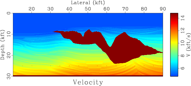
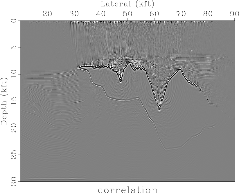
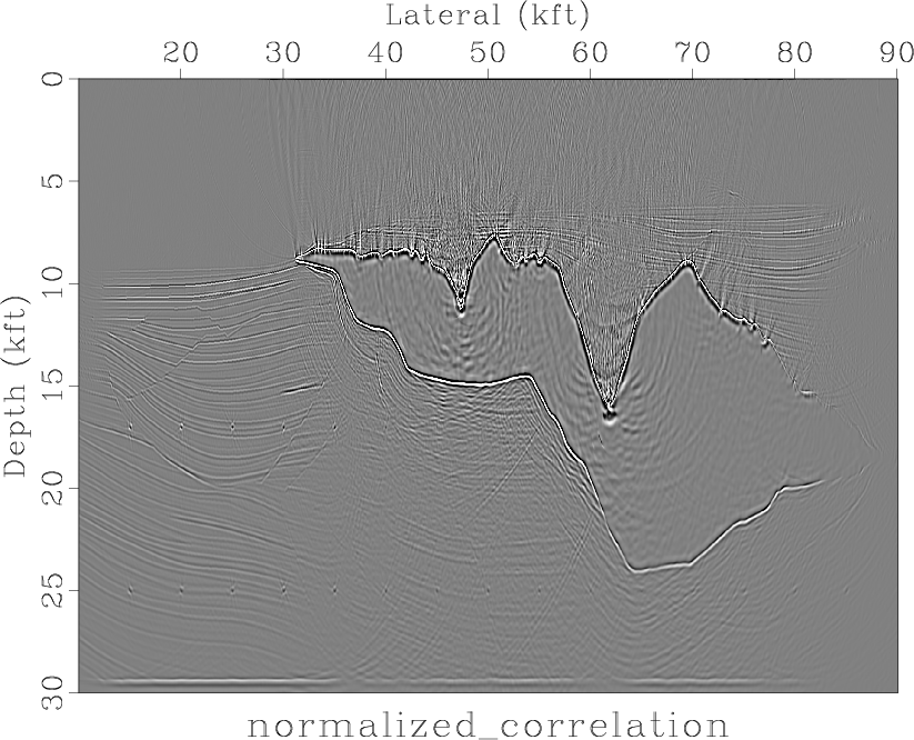
The Sigsbee model is shown in Figure 13. The spatial interval is $\Delta x=\Delta z=25m$ . 55 shots are evenly distributed on the surface of the model. We still perform $nt=13000$ time steps for each shot (301 receivers). Due to the larger model size, 75% boundaries have to be stored with the aid of pinned memory. Our RTM results are shown in Figure 14a and 14b. Again, the resulting image obtained by normalized cross-correlation imaging condition exhibits better resolution for the edges of the salt body and the diffraction points. Some events in the image using normalized cross-correlation imaging condition are more visible, while they have a much lower amplitude or are even completely lost in the image of cross-correlation imaging condition.

sigsbee
Figure 13. The Sigsbee velocity model.

simag1,simag2
Figure 14. RTM result of Sigsbee model using effective boundary saving scheme (staggered grid finite difference). (a) Result of cross-correlation imaging condition. (b) Result of normalized cross-correlation imaging condition.

A numerical tour of wave propagation