|
|
|
|
Plane-wave orthogonal polynomial transform for amplitude-preserving noise attenuation |
Next: Robust slope estimation Up: Theory Previous: Orthogonal polynomial transform
|
|
|
|
Plane-wave orthogonal polynomial transform for amplitude-preserving noise attenuation |
The key question here is how to map the curved events into flattened events. We do the data mapping by a recursively predicting strategy. Each trace in a seismic gather can be predicted using neighbor traces. Given a reference trace, each trace in the gather can predict the reference trace in some ways, e.g., by recursive trace continuation. Ideally, arranging the predicted reference traces (from all other traces) into a gather constructs a flattened gather. Next, we will introduce the theory of how we predict traces following the plane-wave equation, which we call plane-wave trace continuation.
For simplicity, we always treat the first trace in the gather as the reference trace. To flatten the gather, we need to predict the first trace from all other traces and arrange them together. In a brief mathematical way, predicting the first trace from the ![]() th (
th (![]() ) trace can be expressed
) trace can be expressed
Predicting from the ![]() th trace to
th trace to ![]() th trace (or from the
th trace (or from the ![]() th trace to
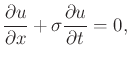
th trace to ![]() th trace) requires solving the plane-wave equation:
th trace) requires solving the plane-wave equation:
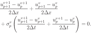
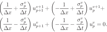
Rearranging the terms in equation 12, we get
Then we have the following point-to-point recursion from ![]() to
to
![]() :
:
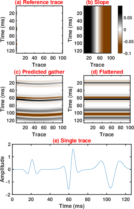
Figure 1 shows an example of the trace prediction process. We start from the first trace in a gather, and predict each trace in the gather from the first trace, following a given local slope field. Figure 1(a) shows the initial status of the trace prediction process, where only the first trace is shown. Following the slope field shown in Figure 1(b), we can predict a complete gather from the first trace using the plane-wave equation. The complete gather is shown in Figure 1(c). It is clear that the morphology of the predicted gather is consistent with the local slope shown in Figure 1(b). Figure 1(d) shows a flattened gather from the curved events shown in Figure 1(c). We flatten the events by predicting the first trace from each trace shown in Figure 1(c). For a clear view of the first trace, we plot it in Figure 1(e).
We then show an example in the presence of random noise. The noisy data is simulated with
![]() , where
, where
![]() is signal, i.e. the solution to a wave equation in some random medium. The signal has a certain mean and variance, and a certain spatial and
temporal correlation structure.
is signal, i.e. the solution to a wave equation in some random medium. The signal has a certain mean and variance, and a certain spatial and
temporal correlation structure.
![]() is the noise, for which, presumably the
expectation
is the noise, for which, presumably the
expectation
![]() is zero. The overall spatial variance of the noise is a certain
number, and its covariance with the signal is zero. The noise is distributed
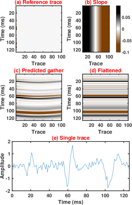
in the 2D plane following a Gaussian rule and has no spatial correlation. Figure 2(a) shows the noisy reference trace. The details of the noisy trace are shown in Figure 2(e). Following a given slope field shown in 2(b), we predict a complete gather from the first trace, and show the gather in Figure 2(c). It can be seen that the noise is preserved during the prediction process. Figure 2(d) shows the flattened gather from Figure 2(c). We can conclude from this test that trace prediction can preserve any component in the starting trace.
is zero. The overall spatial variance of the noise is a certain
number, and its covariance with the signal is zero. The noise is distributed
in the 2D plane following a Gaussian rule and has no spatial correlation. Figure 2(a) shows the noisy reference trace. The details of the noisy trace are shown in Figure 2(e). Following a given slope field shown in 2(b), we predict a complete gather from the first trace, and show the gather in Figure 2(c). It can be seen that the noise is preserved during the prediction process. Figure 2(d) shows the flattened gather from Figure 2(c). We can conclude from this test that trace prediction can preserve any component in the starting trace.
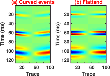
We then use another example to show the amplitude preserving feature of the flattening operator. Figure 3(a) shows a complete gather containing three curved events and amplitude variation along the spatial direction. Figure 3(b) shows the flattened gather from the curved events, where we can see that the amplitude variation is well preserved during the trace prediction process.
|
|---|
|
demo_flat1_r2
Figure 1. Trace prediction for clean data. (a) Reference trace. (b) Slope field. (c) Predicted gather from the reference trace. (d) Flattened gather by predicting the reference trace from each trace in Figure (c). (e) First trace in Figure (a). |
|
|
|
|---|
|
demo_flat2_r2
Figure 2. Trace prediction for noisy data. (a) Reference trace. (b) Slope field. (c) Predicted gather from the reference trace. (d) Flattened gather by predicting the reference trace from each trace in Figure (c). (e) First trace in Figure (a). Note that during trace prediction, the noise is preserved as coherent signal. |
|
|
|
|---|
|
demo_flat3
Figure 3. (a) Curved events. (b) Flattened events by predicting the first trace from each trace in (a). Note that during trace prediction, the amplitude is well preserved. |
|
|
|
|
|
|
Plane-wave orthogonal polynomial transform for amplitude-preserving noise attenuation |
![\begin{displaymath}\begin{split}
&u_{p+1}^{v+1}=
\left(\frac{1}{\Delta x}+\frac{...
...\frac{\sigma_p^v}{\Delta t}\right)u_{p}^{v}\right].
\end{split}\end{displaymath}](img56.png)