Examples

The first example is a synthetic example, as shown in Figure 5. We apply the Karhunen-Loève (KL) filtering method (Jones and Levy, 1987) and the proposed method to a flattened dataset with strong amplitude variation. Figure 5a shows the clean data, and Figure 14b shows the noisy data. Figures 5b and 5c show the denoised data using the KL filtering method and the proposed method, respectively. Figures 5e and 5f show the removed random noise using two approaches. We can observe clearly from Figures 5b and 5c that the KL filtering causes significant damages to the events, while the proposed method preserves the amplitude-variation details successfully.

In order to compare the amplitude between different seismic profiles in detail, we compare the amplitude for a single trace from each section shown in Figure 5. The trace is chosen as the 20th trace in each section of Figure 5. The comparison is presented in Figure 6a. A zoom-in comparison is shown in Figure 6b. The black line is from the clean data. The red line is from the noisy data. The blue line corresponds to the KL method. The green line corresponds to the proposed method. It is apparent that the green line is very close to the black line while the blue line deviates from the black line too much in most areas. This trace amplitude comparison further confirms the superior performance of the proposed algorithm.

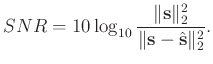
In order to numerically compare the denoising performance, we use the commonly used signal-to-noise ratio (SNR) defined as follows to quantitatively measure the performance (Chen and Fomel, 2015b):

$$SNR=10\log_{10}\frac{\Arrowvert \mathbf{s} \Arrowvert_2^2}{\Arrowvert \mathbf{s} -\hat{\mathbf{s}}\Arrowvert_2^2}.$$ (18)

where $\mathbf{s}$ denotes the noise-free data and $\hat{\mathbf{s}}$ denotes the denoised data. In addition, to quantitatively measure the noise removal in the case of no discernable signal damage, we define the metric as the root-mean-square (RMS)

$$RMS=\Arrowvert\mathbf{n}\Arrowvert_2,$$ (19)

where $\mathbf{n}$ denotes the removed noise. Although the amplitude range varies a lot for different data sets, the RMS metric provides us a quantitative way to evaluate the noise removal performance for one specific data set among different denoising methods, e.g., how much better method A performs than method B.

In order to compare the performance of two methods in different noise level. We increase the variance of noise from 0.1 to 1.0, and calculate the SNRs of denoised data of both methods and show them in Table 1. To see the varied SNRs more vividly, we plot the data from Table 1 in Figure 7. The black line shows the SNRs varying with input noise variances. The red line shows the SNRs corresponding to the KL method. The blue line shows the SNRs of the OPT method. It is obvious that both methods obtain large SNR improvement for all noise levels and the SNRs of the OPT method are always higher than the KL method. We can also observe clearly that the difference between the proposed OPT method and the KL method increases as noise variance becomes larger, which indicates that the proposed method outperforms the KL method more when the seismic data becomes noisier.

Table 1: Comparison of SNRs in dB for different input noise level. The diagram corresponding to this table is shown in Figure 7.

Noise variance	Input data (dB)	KL (dB)	OPT (dB)
0.1	2.60	13.08	17.58
0.2	-3.42	6.92	11.56
0.3	-6.94	3.05	8.04
0.4	-9.44	0.19	5.54
0.5	-11.38	-1.89	3.60
0.6	-12.97	-3.54	2.02
0.7	-14.30	-4.94	0.68
0.8	-15.46-	-6.17	-0.48
0.9	-16.49	-7.26	-1.50
1.0	-17.40	-8.25	-2.42

For computational cost comparison, the KL method takes 0.62s for processing the data shown in Figure 14b while the proposed algorithm takes 0.01s. The data contains 151 samples and 61 traces. The computation is done on a PC station equipped with an Intel Core i7 CPU clocked at 3.1 GHz and 16 GB of RAM. Note that both KL and OPT methods require the events to be flattened in order to obtain the best performance, thus we only compare the cost difference in the filtering stage.

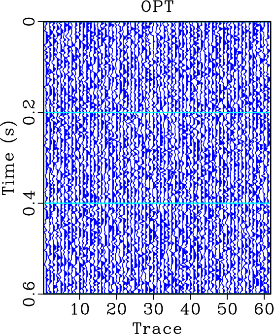
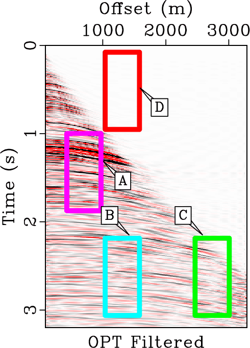
The second example is a pre-stack field data example. Figure 8a shows the original data. Figures 8b, 8c, and 8d show the denoised data using EMD method, KL method, and the proposed method, respectively. Figures 9 shows the removed noise sections using three approaches. Figure 9a shows that some low-frequency energy is damaged while Figure 9c shows that the removed noise is stronger. In this example, the calculated RMSs for Figures 9a(a), 9a(b), and 9a(c) are 389.49, 449.22, and 506.26, respectively. Thus, the proposed method removes 12.7% more noise than the KL method and 30.0% more noise than the EMD method.

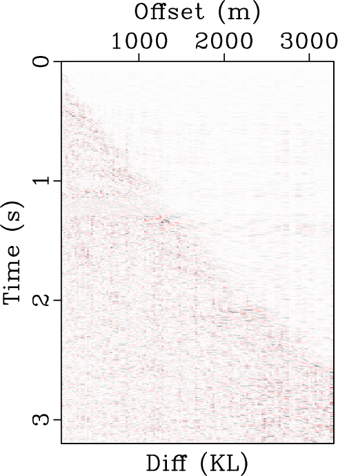
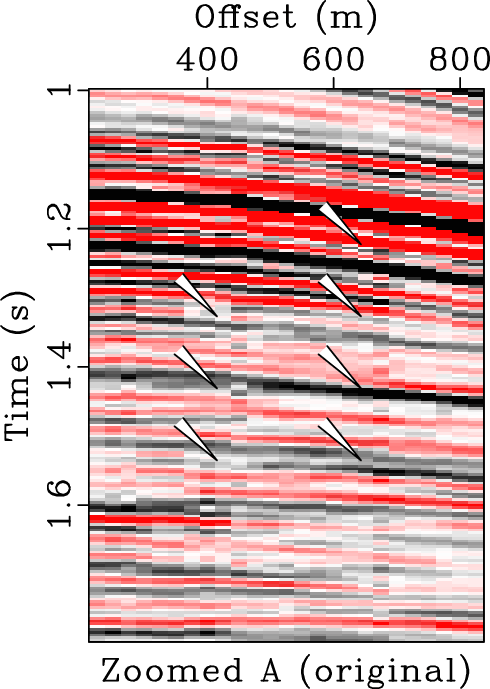
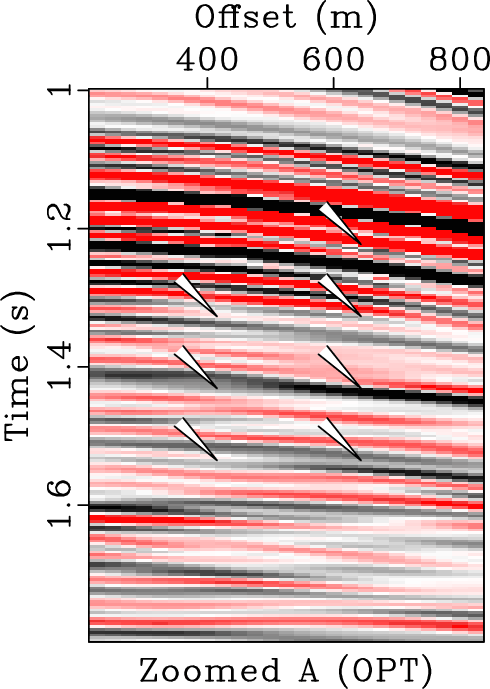
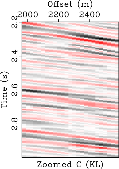
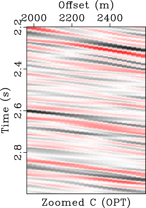
In order to comprehensively compare three different approaches, we zoomed four frame boxes (A,B,C,D) to show the detailed difference. Figure 10 shows the comparison from frame box A. It is obvious that the KL approach causes some residual noise while EMD and OPT approaches obtain good results, more careful observation can show that the proposed method can obtain a more coherent image. Figure 11 shows the comparison for frame box B. It is obvious that OPT method obtains the cleanest result. Figure 12 shows the comparison for frame box C. It is still obvious that OPT method can make the events more coherent and more importantly, preserve the amplitude-variation-with-offsets (AVO) details well. Figure 13 shows the comparison for frame box D. Both Figures 13b and 13c show obvious amplitude artifacts while the OPT result in Figure 13d shows nearly zero amplitude in the zoomed section.

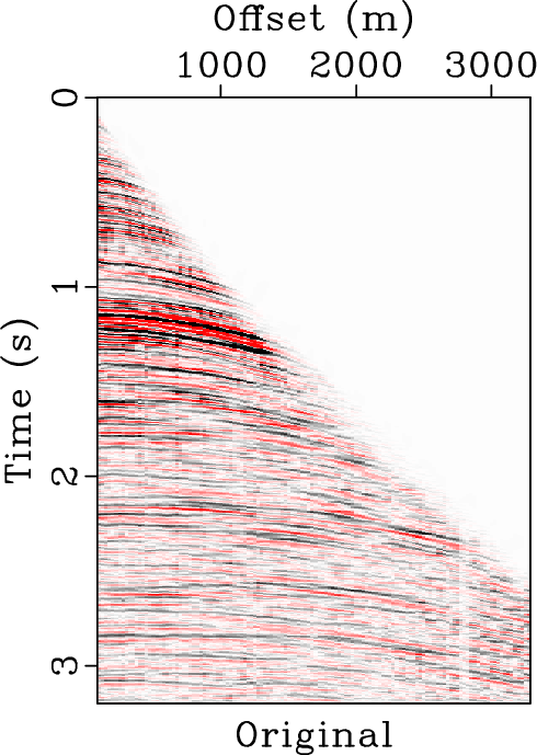
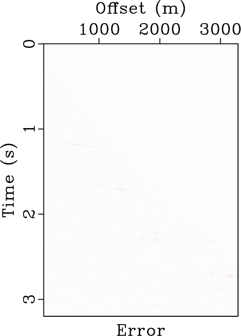
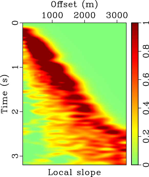
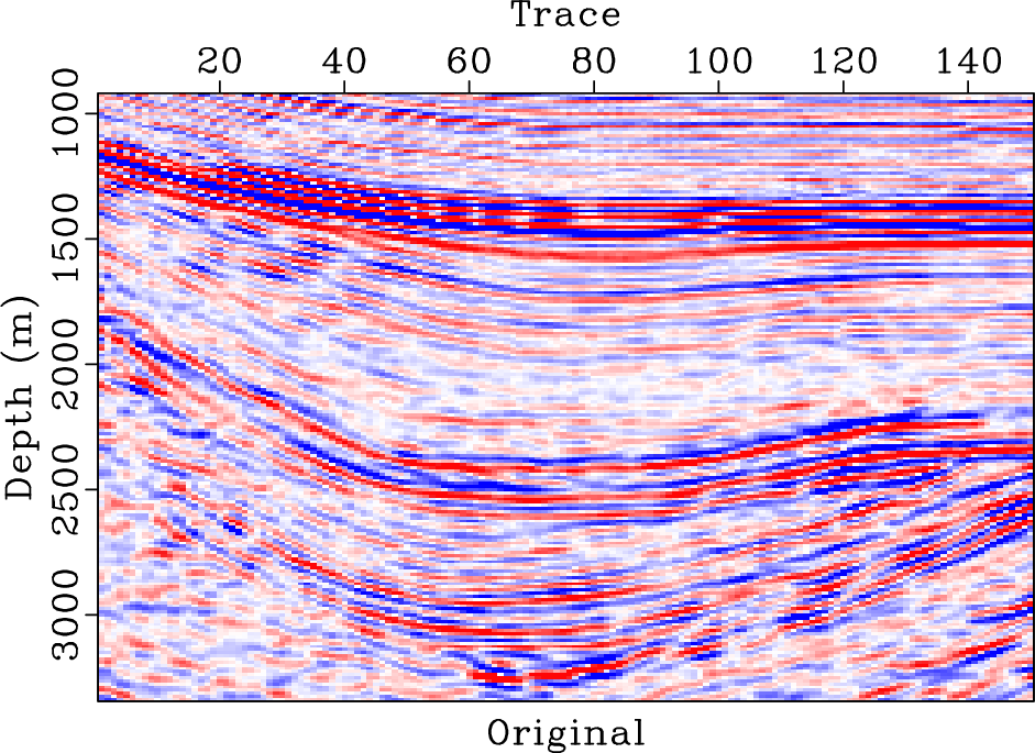
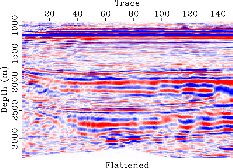
For this example, we also demonstrate the flattening process in Figure 14. Figure 14b shows the flattened gather from the original data shown in Figure 14a (or Figure 8a). It is clear that most events have been flattened well. Figure 14c shows the reconstructed data from the inverse flattening. The data is almost the same as the original data. Figure 14d shows the difference between the reconstructed data and the original data. The error section is almost zero everywhere, which demonstrates that the flattening process does not introduce extra error. Figure 15 shows the slope estimated from the original data. We also show a detailed comparison between different data in the flattened dimension in Figure 16. A zoomed comparison among the flattened gathers after filtering is shown in Figure 17, where we can conclude that the proposed method obtains the smoothest result while best preserving the reflection amplitude.

The next example is a real post-stack seismic image shown in Figure 18a. There are 140 spatial traces and 194 temporal samples. The seismic image contains highly curved events and the amplitude along the events is not continuous, which will make the seismic interpretation difficult. After using three approaches, the EMD method, the KL method, and the proposed method, the denoised images are shown in Figures 18b, 18c, and 18d, respectively. It is obvious that the proposed OPT based filtering approach can obtain a well smoothed seismic image with the continuity and the amplitude of events enhanced greatly. The EMD based approach, however, cannot effectively smooth the seismic events, and still leaves a lot of discontinuity in the image. The KL filtering approach obtains a much better filtering performance compared with the EMD based approach, however, it is not as successful as the performance of the proposed OPT based approach.

We can find the mechanism that caused the tremendous difference of denoised images from the comparison in the flattened domain, as shown in Figure 19. It is even more obvious that the OPT based approach obtains a nearly perfect smoothing along the flattened images (equivalent to along the structure in the original domain). The EMD based approach can achieve some smoothing, but remains less continuous than both KL and OPT based approaches. In this example, the calculated RMSs of removed noise are 0.015 for EMD method, 0.016 for KL method, and 0.019 for the proposed method. Thus, the proposed method removes 18.7% more noise than the KL method and 25.0% more noise than the EMD method.

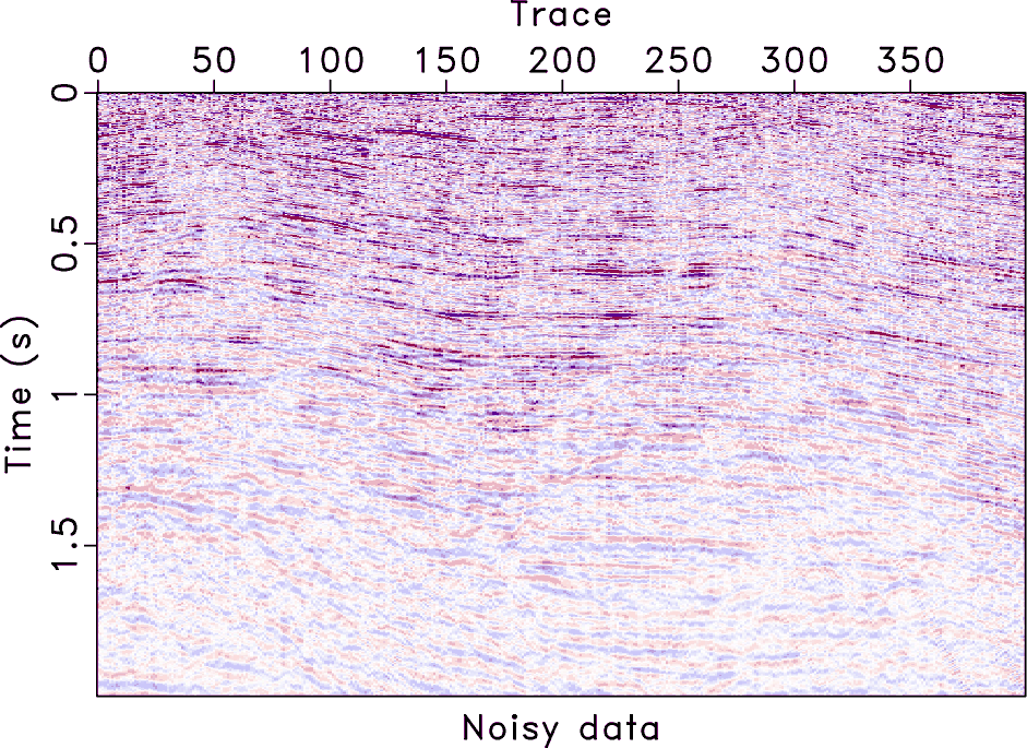
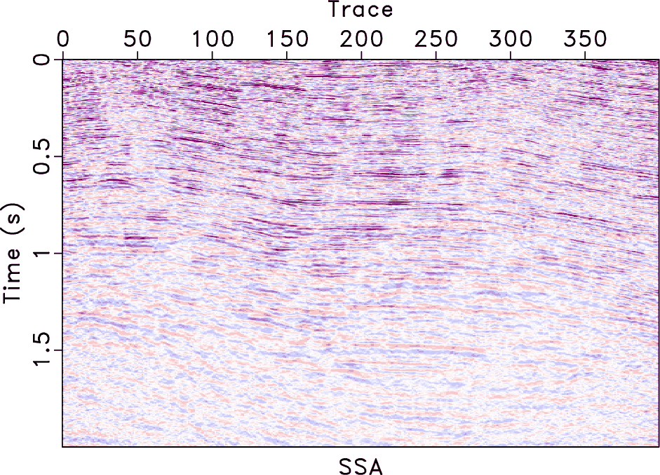
The next field data example is shown in Figure 20a, which is also a post-stack data and contains weak seismic reflection events. Figures 20b, 20c, and 20d show the denoised results using three different methods. For this example, we further compare the performance of the proposed method with that of the $f-x$ predictive filtering method and the singular-spectrum analysis (SSA) method (Vautard et al., 1992). Figure 21 shows the corresponding noise sections. For this example, it seems that all three methods obtain much improved results and the performance of different methods is quite similar. In order to compare the performance in detail and more fairly, we plot the $F-K$ spectra of different denoised results. The $F-K$ spectrum of the raw data is shown in Figure 22a. The $F-K$ spectra corresponding to different methods are shown in Figures 22b, 22c, and 22d. Comparing the $F-K$ spectra of different methods and $F-K$ spectrum of the raw data, it is easy to find that both $f-x$ predictive filtering method and the proposed method preserve the useful signals well, but the $f-x$ predictive filtering method has some residual spectrum energy around the edges (large wavenumber components). SSA method causes significant damages to useful signals.

In this example, we also calculate the local similarity between the denoised data and removed noise for different methods. The local similarity is an effective way to detect the lost signals in the removed noise. High local similarity indicates that in the noise section, there are significantly similar components as the useful signals, i.e., there is lost energy in the noise. The calculation of local similarity is provided in Appendix B. The local similarity maps for different methods are shown in Figure 23, where we can clearly observe the high similarity anomalies in the $f-x$ predictive filtering and SSA results. Although there are also some similarity anomalies in the result from the proposed method, the similarity value is relatively lower than the other two methods. From this test we conclude that the proposed method causes less damage to useful energy.

We also plot a comparison of the average spectrum of all the traces for different data in Figure 24. The green line corresponds to the proposed approach. The red line corresponds to $f-x$ predictive filtering method. The blue line corresponds to the SSA method. It is quite obvious that the energy preservation of the proposed method in signal frequency band (20$\sim$60 Hz) is quite successful. The proposed method mitigates more high-frequency noise than $f-x$ predictive filtering method, which confirms the observation from Figure 22. We admit that the high-frequency noise of the proposed method is slightly more than the SSA method. However, the proposed method preserves more useful energy than the other two methods in the spectrum. This field data further confirms the superior performance of the presented algorithm.

In this example, to compare the noise removal performance, we need to make sure the removed noise sections do not contain discernable signal energy, as required by the metric defined in equation 19, and have to adjust the parameters for the $f-x$ and SSA methods. The denoised data and the removed noise sections using the adjusted parameters are shown in Figure 25. In this case, the calculated RMSs for Figures 25(d), 25(e), and 25(f) are 0.059, 0.071, and 0.086, respectively. Thus, the proposed method removes 21.1% more noise than the SSA method and 38.0% more noise than the $f-x$ method.

flat-c,flat-kl,flat-opt,flat,flat-kl-dif,flat-opt-dif
Figure 5. Synthetic example. (a) Clean data. (b) Denoised data using KL filtering. (c) Denoised data using the proposed method. (d) Noisy data. (e) Noise section corresponding to (b). (f) Noise section corresponding to (c).

flat-ss,flat-ss-z
Figure 6. Comparison of the 20th trace amplitude of each seismic gather in Figure 5. The black line is from the clean data. The red line is from the noisy data. The blue line corresponds to the KL method. The green line corresponds to the proposed method. (a) Comparison of the whole trace. (b) Zoom-in comparison. Note that the black and green lines are very close to each other, thus the reconstruction error using the proposed approach is much less than the traditional method for most parts.

flat-snrs
Figure 7. SNR diagrams of synthetic example.

gath0,flat-emd-rec0,flat-kl-rec0,flat-opt-rec0
Figure 8. Denoising comparison. (a) Raw noisy data. (b) Filtered using EMD method. (c) Filtered using KL method. (d) Filtered using the proposed method.

dif,dif-kl,dif-opt
Figure 9. Noise comparison. (b) Removed noise using EMD method. (b) Removed noise using KL method. (c) Removed noise using the proposed method.

zooma-1z,zooma-2z,zooma-4z,zooma-5z
Figure 10. Zoomed frame box A from Figure 8. (a) Zoomed noisy field data. (b) Zoomed filtered data using EMD method. (c) Zoomed filtered data using KL method. (d) Zoomed filtered data using the proposed method.

zoomb-1,zoomb-2,zoomb-4,zoomb-5
Figure 11. Zoomed frame box B from Figure 8. (a) Zoomed noisy field data. (b) Zoomed filtered data using EMD method. (c) Zoomed filtered data using KL method. (d) Zoomed filtered data using the proposed method.

zoomc-1,zoomc-2,zoomc-4,zoomc-5
Figure 12. Zoomed frame box C from Figure 8. (a) Zoomed noisy field data. (b) Zoomed filtered data using EMD method. (c) Zoomed filtered data using KL method. (d) Zoomed filtered data using the proposed method.

zoomd-1,zoomd-2,zoomd-4,zoomd-5
Figure 13. Zoomed frame box D from Figure 8. (a) Zoomed noisy field data. (b) Zoomed filtered data using EMD method. (c) Zoomed filtered data using KL method. (d) Zoomed filtered data using the proposed method.

gath,flat,gath-rec,gath-dif
Figure 14. Pre-stack field data example. (a) Field data. (b) Flattened field data. (c) Reconstructed field data. (d) Reconstruction error.

dip
Figure 15. Local slope estimation of the pre-stack field data.

flat0,flat-emd0,flat-kl0,flat-opt0
Figure 16. Denoising comparison in the flattened dimension. (a) Raw noisy data. (b) Filtered using EMD method. (b) Filtered using KL method. (c) Filtered using the proposed method.

zoom-1,zoom-2,zoom-4,zoom-5
Figure 17. Zoomed sections from Figure 16. (a) Zoomed noisy field data. (b) Zoomed filtered data using EMD method. (c) Zoomed filtered data using KL method. (d) Zoomed filtered data using the proposed method.

post-gath,post-emd-rec,post-kl-rec,post-opt-rec
Figure 18. First post-stack field data example. (a) Field data. (b) Filtered data using EMD method. (c) Filtered data using KL method. (d) Filtered data using the proposed method.

post-flat,post-flat-emd,post-flat-kl,post-flat-opt
Figure 19. Comparison in the flattened domain. (a) Field data. (b) Filtered data using EMD method. (c) Filtered data using KL method. (d) Filtered data using the proposed method.

f2,f2-fx,f2-ssa,f2-opt
Figure 20. Denoising comparison for the second post-stack field data. (a) The second post-stack field data. (b) Filtered data using $f-x$ predictive filtering. (c) Filtered data using SSA. (d) Filtered data using the proposed method.

f2-fx-dif,f2-ssa-dif,f2-opt-dif
Figure 21. Noise comparison for the second post-stack field data. (a) Removed noise using $f-x$ predictive filtering. (b) Removed noise using SSA. (c) Removed noise using the proposed method.

f2-f,f2-fx-f,f2-ssa-f,f2-opt-f
Figure 22. Spectra comparison. (a)Spectrum of the second post-stack seismic data. (b) Spectrum using $f-x$ predictive filtering. (c) Spectrum using SSA. (d) Spectrum using the proposed method.

f2-fx-simi,f2-ssa-simi,f2-opt-simi
Figure 23. Comparison of local similarity between denoised data and removed noise. (a) Local similarity using $f-x$ predictive filtering. (b) Local similarity using SSA. (c) Local similarity using the proposed method.

f2-fs
Figure 24. Comparisons of the average spectrum of all the traces. The black line denotes the average spectrum of raw data. The green line corresponds to the proposed approach. The red line corresponds to $f-x$ predictive filtering method. The blue line corresponds to the SSA method.

f2-fx2,f2-ssa2,f2-opt2,f2-fx2-dif,f2-ssa2-dif,f2-opt2-dif
Figure 25. Comparison for the second post-stack field data after adjusting the parameters. (a) Filtered data using $f-x$ predictive filtering. (b) Filtered data using SSA. (c) Filtered data using the proposed method. (d) Removed noise using $f-x$ predictive filtering. (e) Removed noise using SSA. (f) Removed noise using the proposed method. In this case, the calculated RMSs for (d),(e), and (f) are 0.059, 0.071, and 0.086, respectively. Thus, the proposed method removes 21.1% more noise than the SSA method and 38.0% more noise than the $f-x$ predictive filtering method.