Examples

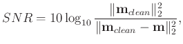
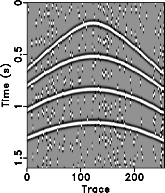
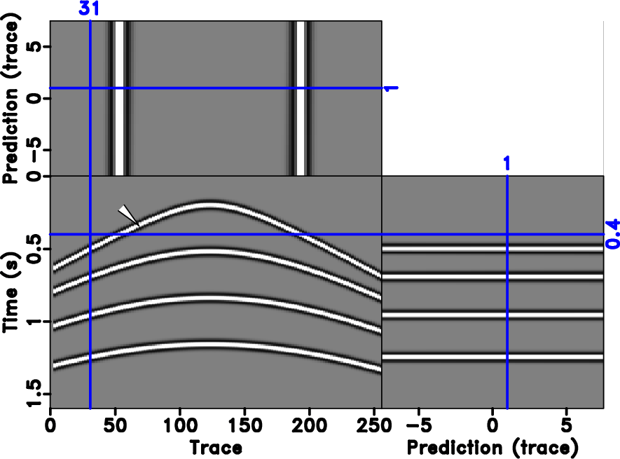
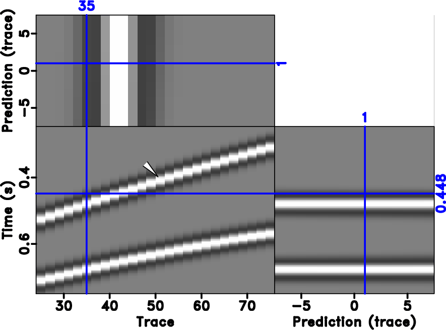
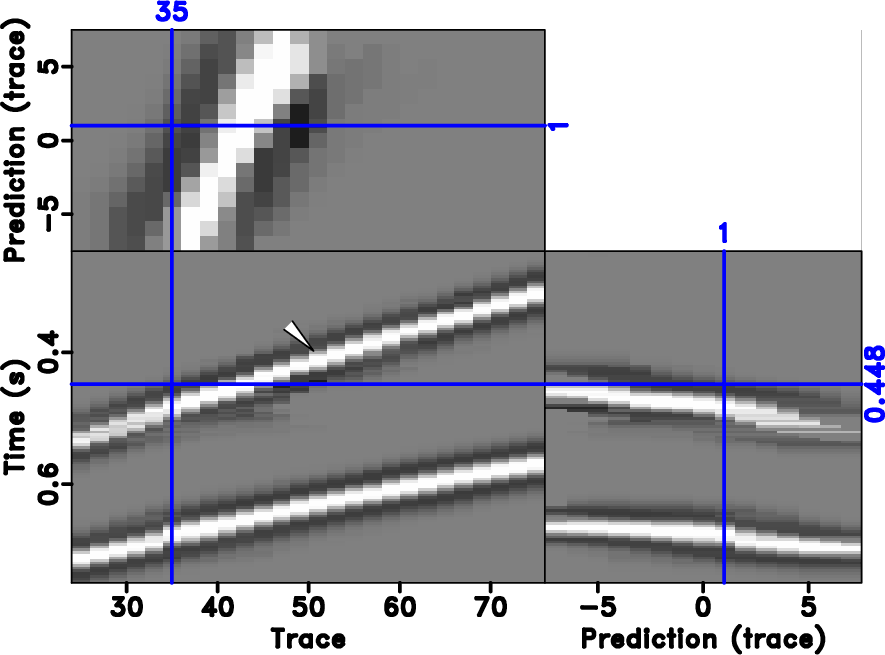
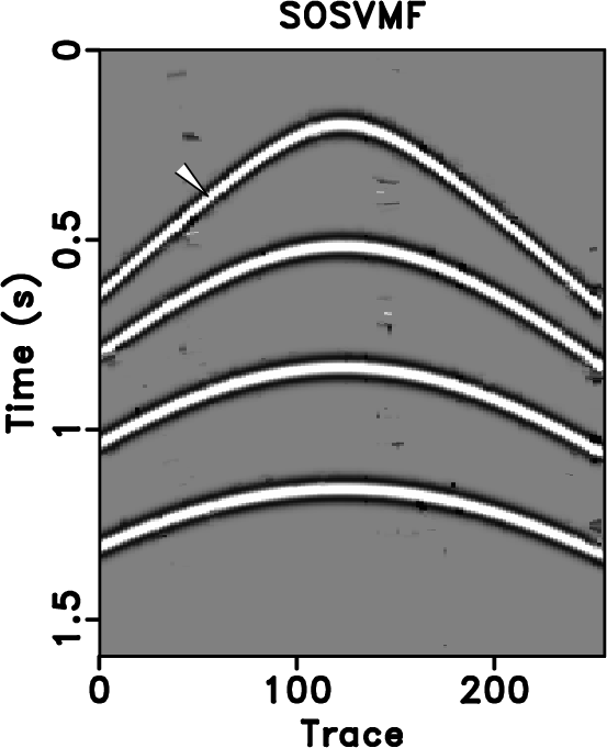
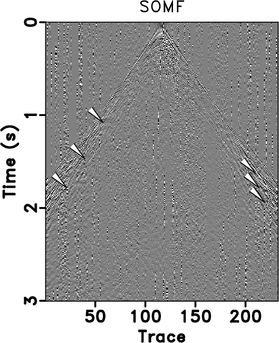
We first test the structure-oriented space-varying median filter method on a simple synthetic example. Figure 8a shows a simple hyperbolic synthetic example. We create the data using the Kirchhoff 2-D/2.5-D modeling method with analytical Green's functions, introduced in Haddon and Buchen (1981). Figure 8b shows the noisy data with some blending noise. Figure 8c shows the slope estimated from the clean data and Figure 8d shows the slope estimated from the noisy data. The strong noise makes the slope estimation inaccurate. Figures 9a and 9b show a comparison between the flattened unblended data using accurate slope and flattened blended data using inaccurate local slope, respectively. From Figure 9a, we can observe that the data is flattened well locally using the accurate local estimation (from the unblended data). From Figure 9b, it is obvious that the events in the flattened dimension are not horizontal, which indicates an imperfect local flattening. Figures 9c and 9d show a comparison between the filtered data using the median filter and space-varying median filter, respectively. Both median filter and space-varying median filter are applied along the flattened dimension (along the “prediction” axis). It is clear that some energy is damaged using the median filter and the signals are preserved well using the space-varying median filter method, as indicated by the white arrow in Figure 9. For a clearer comparison, we show the zoomed data of Figure 9 in Figure 10. Figure 11 shows a deblending comparison between the median filter, space-varying median filter, structure-oriented median filter, and structure-oriented space-varying median filter methods, respectively. From Figure 11, we can see that the traditional median filter results in the largest damages, which is followed by space-varying median filter. structure-oriented median filter preserves most signals but still causes some damages, as indicated by the white arrow. Among the four results, the structure-oriented space-varying median filter result is the best in preserving dipping energy and rejecting spike-like blending noise. A zoomed comparison of Figure 11 is shown in Figure 11. Figure 13 shows the removed blending noise corresponding to the four aforementioned methods, which confirms the observation from Figure 11 that median filter, space-varying median filter, and structure-oriented median filter all result in more or less signal leakage (Chen and Fomel, 2015) to the noise sections. In this example, we use the signal-to-noise ratio (SNR) to quantitatively compare the deblending performance using different methods:

$$SNR=10\log_{10}\frac{\Arrowvert \mathbf{m}_{clean} \Arrowvert_2^2}{\Arrowvert \mathbf{m}_{clean} -\mathbf{m}\Arrowvert_2^2},$$ (9)

where $\mathbf{m}_{clean}$ denotes the exact solution, or the unblended data. $\mathbf{m}$ denotes the deblended data. Using this metic, we calculate the SNRs of the blended data, deblended data using median filter, space-varying median filter, structure-oriented median filter, and structure-oriented space-varying median filter methods as 1.62 dB, 5.46 dB, 8.63 dB, 12.46 dB, and 16.55 dB, respectively. The structure-oriented space-varying median filter method obtains the highest SNR.

hyper,hyper-n,hdip,hdip-n
Figure 8. (a) Clean data. (b) Noisy data with spike-like blending noise. (c) Estimated slope from the clean data. (d) Estimated slope from the noisy data.

hflat0,hflat-n0,hflat-n-mf0,hflat-n-svmf0
Figure 9. (a) Flattened dimension of the clean data using the accurate slope. (b) Flattened dimension of the noisy data using the inaccurate slope. (c) Filtered data using median filter in the flattened domain. (b) Filtered data using space-varying median filter in the flattened domain.

hflat-z0,hflat-n-z0,hflat-n-mf-z0,hflat-n-svmf-z0
Figure 10. Zoomed comparison of Figure 9. (a) Flattened dimension of the clean data using the accurate slope. (b) Flattened dimension of the noisy data using the inaccurate slope. (c) Filtered data using median filter in the flattened domain. (b) Filtered data using space-varying median filter in the flattened domain.

hyper-mf0,hyper-svmf0,hyper-somf0,hyper-sosvmf0
Figure 11. (a) Deblended data using median filter. (b) Deblended data using space-varying median filter. (c) Deblended data using structure-oriented median filter. (d) Deblended data using structure-oriented space-varying median filter. Note that since all median filters are only applied once, so there are several spikes left. The one-step processing is efficient but can be improved through multiple iterations (e.g., in iterative deblending).

hyper-mf-z0,hyper-svmf-z0,hyper-somf-z0,hyper-sosvmf-z0
Figure 12. Zoomed comparison of Figure 11. (a) Deblended data using median filter. (b) Deblended data using space-varying median filter. (c) Deblended data using structure-oriented median filter. (d) Deblended data using structure-oriented space-varying median filter.

hyper-mf-n,hyper-svmf-n,hyper-somf-n,hyper-sosvmf-n
Figure 13. (a)-(d) Removed blending noise sections corresponding to Figures 11 (a)-(c), respectively.

shot-n,sdip-n
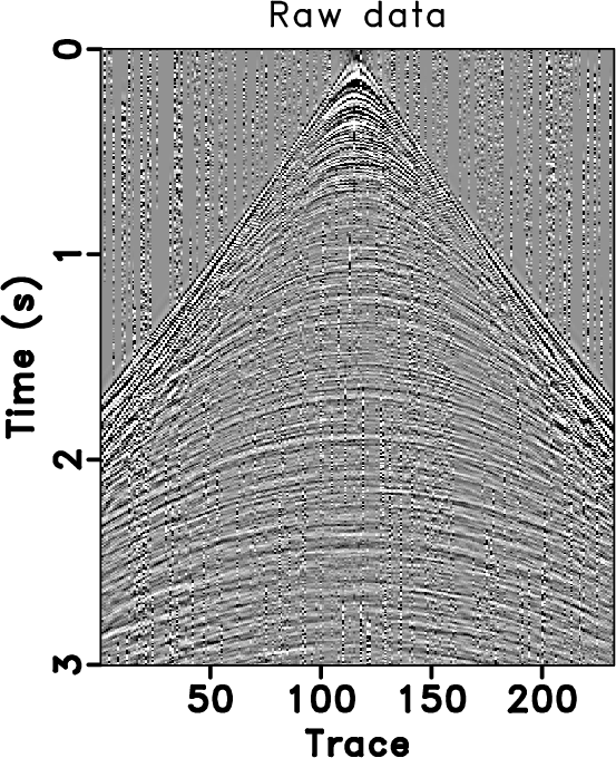
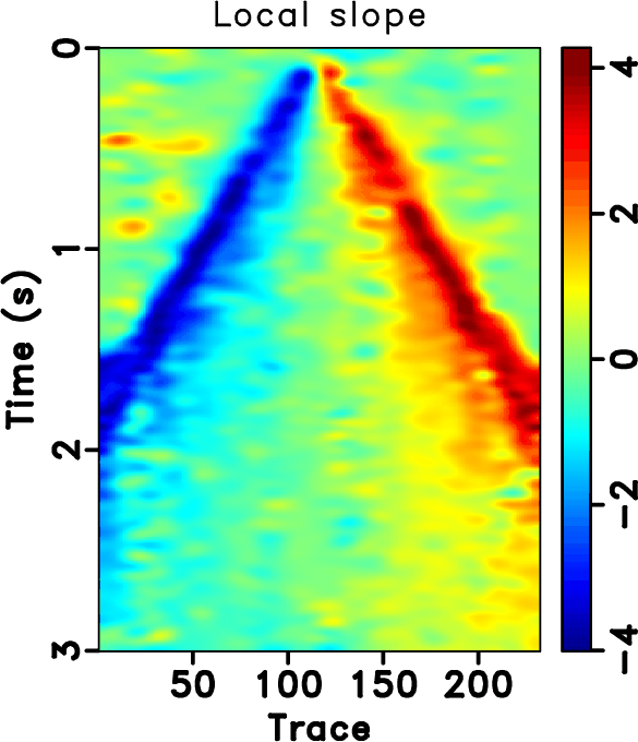
Figure 14. (a) Simultaneous source data. (b) Slope estimated from the raw data.

shot-mf,shot-svmf,shot-somf,shot-sosvmf
Figure 15. (a) Deblended data using median filter. (b) Deblended data using space-varying median filter. (c) Deblended data using structure-oriented median filter. (d) Deblended data using structure-oriented space-varying median filter.

shot-mf-n-0,shot-svmf-n-0,shot-somf-n-0,shot-sosvmf-n-0
Figure 16. (a) Removed blending noise using median filter. (b) Removed blending noise using space-varying median filter. (c) Removed blending noise using structure-oriented median filter. (d) Removed blending noise using structure-oriented space-varying median filter.

shot-mf-s,shot-svmf-s,shot-somf-s,shot-sosvmf-s
Figure 17. A comparison of local similarity between deblended data and removed blending noise. (a) Local similarity using median filter. (b) Local similarity using space-varying median filter. (c) Local similarity using structure-oriented median filter. (d) Local similarity using structure-oriented space-varying median filter.

The next example is a field data test. Figure 14a shows the a common receiver gather that contains blending noise. The data is a benchmark testing data shared by BGP, China. Figure 14b shows the local slope map calculated from the raw data using the plane-wave destruction algorithm. The deblended results using four methods are shown in Figure 15. The removed blending noise corresponding to the four methods are shown in Figure 16. Combining Figures 15 and 16, it is easy to conclude that both median filter and space-varying median filter methods cause a large amount of damaged energy, the structure-oriented median filter method causes relatively less damaged energy around the large-offset areas, and the structure-oriented space-varying median filter method causes negligible damaged energy. Note that the signal damages are highlighted by the white arrows in Figure 16. In this example, the exact solution is unknown, thus we cannot use the quantitative metric that is used previously to compare the performance quantitatively. But we use the local similarity to measure the signal damage. The local similarity between the denoised (deblended) and removed noise sections are calculated to detect the signal damage for a denoising (deblending) algorithm, as proposed in Chen and Fomel (2015). High anomalies in the local similarity map indicates a more servere signal damage. The most distinct advantage of the local similarity measure is that it can measure the signal damage in a local and vivid way. Figure 17 show the four local similarity maps for the four methods. The comparison of local similarity shows vividly that all median filter, space-varying median filter, and structure-oriented median filter methods cause a large amount of damaged signals in the noise and the signal damage using the structure-oriented space-varying median filter method is the least. It is worth mentioning that some shallow reflections are not well predicted. This is likely because of the curvature of the events and the linearity of the process.

Next, we simulate a multi-receivers 2D simultaneous source separation test. In this test, we want to test how the structure-oriented space-varying median filter method performs when embedded into an iterative deblending framework. Figure 18a shows the acquisition geometry of the 2D test. The red dots denote 120 evenly spaced shot locations on the surface. The blue inverted triangles denote 120 evenly spaced receivers. Note that in this acquisition geometry, the simultaneous shooting and traditional shooting only differ in the shot schedule (Abma, 2014). Figure 18b shows the shot schedules for the traditional and the faster simultaneous source shooting. It is worth mentioning here that although there is only one source in this test, the faster shooting scheduling results in an overlapping subsurface reflection responses in time, which is still considered as simultaneous shooting (Abma et al., 2015). From the shot schedule, it is obvious that the shooting time for the simultaneous source acquisition is almost half of the traditional acquisition and thus saves about half of the traditional acquisition cost. In this example, we use a relatively realistic field dataset to mimic the unblended data ( $\mathbf{m}$ in equation 7), as shown in Figure 19a. The data is a marine data set provided by BGP China. The size of the data is $1500\times 120\times120$ (in time-shot-receiver domain). Figure 19b shows the blended data ( $\mathbf{d}$ in equation 7). It is clear that the blending noise appears to be spatially incoherent in the common receiver domain (along the shot axis) and spatially coherent in the common shot domain (along the receiver axis). Figure 20a shows iteratively deblended data using the rank-constrained shaping regularization framework (Chen et al., 2014; Zu et al., 2017c). The iterative deblending is carried out in each common receiver gather based on the coherency difference between useful signals and interfering noise. For the rank-constrained inversion, we use local windows with the size of $200\times 20$ ( time$\times$   space). A constant rank strategy is used for each window with $rank=2$. We obtain the result shown in Figure 20a with 40 iterations. Comparing the rank-constrained deblended data with the blended data, it is clear that most blending noise is removed. However, there is still much residual noise. By cascading the structure-oriented space-varying median filter and the rank filter based on the iterative shaping regularization framework, as expressed by equations 8, we obtain a much improved deblended result, as shown in Figure 20b. During the inversion, we linearly decrease the filter length from 11 points to 0. A comparison between the two deblended data in Figure 20 confirms the effectiveness of the structure-oriented space-varying median filter method in improving iterative deblending. Figure 21 shows the deblending error for the traditional method and the proposed method. The deblending error means the difference between the unblended data (exact solution) and the deblended data. From Figure 21, it is obvious that the deblending error for the proposed method is negligible while the error for the rank-reduction method is very large. Figure 22 shows the removed noise corresponding to the two methods, note that the interfering shots are coherent in the second spatial dimension.. For evaluating the signal damages of this example, we calculate the local similarity between the deblended data and the noise and show them in Figure 23, where much larger local similarity anomalies are shown in the similarity map corresponding the traditional method. To compare the amplitude preservation in detail, we plot a trace-by-trace comparison in Figure 24a. The black line is from the unblended data. The red line is from the blended data. The magenta line corresponds to the rank-constrained method. The green line corresponds to the proposed method. It is salient that the black and green lines are very close to each other, thus the deblending error using the proposed approach is much less than the traditional method for most parts. In order to compare the hybrid method with the structure-oriented space-varying median filter and the hybrid with the structure-oriented median filter, we also have a inversion test using the structure-oriented median filter. The deblended data is shown in Figure 25. It is obvious that the hybrid method with the structure-oriented median filter causes much higher deblending error.

geom,shottime
Figure 18. (a) Acquisition geometry. The red dots denote shot locations and blue inverted triangles denote receivers. The simultaneous shooting and the traditional shooting only differ in the shot schedule. (b) Shot schedule. Note that the shot schedule is just for testing purpose and does not represent a real field deployment. In the test, the speed of a shooting vessel is assumed to be sufficiently large. In practice, the shot sampling would be much higher than the testing case, which is 0.05 km.

d3d,b3d
Figure 19. Shot-receiver data example. (a) Unblended data. (b) Blended data.

m3d,im3d
Figure 20. A comparison between iterative deblending performance. (a) Iteratively deblended data using the rank-constrained method. (b) Deblended data using the proposed method.

m3d-e,im3d-e
Figure 21. A comparison between deblending error. (a) Error corresponding to the traditional rank-constrained method. (b) Error corresponding to the proposed method.

m3d-n,im3d-n
Figure 22. A comparison between removed blending noise. (a) Removed blending noise corresponding to the traditional rank-constrained method. (b) Removed blending noise corresponding to the proposed method.

m3d-s,im3d-s
Figure 23. A comparison between local similarity comparison. (a) Local similarity corresponding to the traditional rank-constrained method. (b) Local similarity corresponding to the proposed method. Note the much larger similarity anomaly shown in (a).

trace,trace-z
Figure 24. Single trace comparison. The black line is from the unblended data. The red line is from the blended data. The magenta corresponds to the rank-constrained method. The green line corresponds to the proposed proposed method. Note that the black and green lines are very close to each other, thus the deblending error using the proposed approach is much less than the traditional method for most parts. (a) Comparison in the original size. (b) Comparison in a zoomed view.

im3d-2,im3d-e-2
Figure 25. Deblending performance using the hybrid method with structure-oriented median filter. (a) Deblended data. (b) Deblending error. Note that the deblending error in this case is much higher than the hybrid method with structure-oriented space-varying median filter (Figure 21b).