Downward continuation

Downward continuation with Fourier transform

One of the main ideas in Fourier analysis is that an impulse function (a delta function) can be constructed by the superposition of sinusoids (or complex exponentials). In the study of time series this construction is used for the impulse response of a filter. In the study of functions of space, it is used to make a physical point source that can manufacture the downgoing waves that initialize the reflection seismic experiment. Likewise observed upcoming waves can be Fourier transformed over $t$ and $x$.

Recall in chapter , a plane wave carrying an arbitrary waveform, specified by equation (). Specializing the arbitrary function to be the real part of the function $\exp [ - i \omega (t-t_0 ) ]$ gives

$$\hbox{moving cosine wave} = \cos \left[ \omega \lef... ... +\ {z \over v } \cos \theta - t \right) \right]$$ (8)

Using Fourier integrals on time functions we encounter the Fourier kernel $\exp(-i\omega t)$. To use Fourier integrals on the space-axis $x$ the spatial angular frequency must be defined. Since we will ultimately encounter many space axes (three for shot, three for geophone, also the midpoint and offset), the convention will be to use a subscript on the letter $k$ to denote the axis being Fourier transformed. So $k_x$ is the angular spatial frequency on the $x$-axis and $\exp ( i k_x x )$ is its Fourier kernel. For each axis and Fourier kernel there is the question of the sign before the $i$. The sign convention used here is the one used in most physics books, namely, the one that agrees with equation (7.8). Reasons for the choice are given in chapter . With this convention, a wave moves in the positive direction along the space axes. Thus the Fourier kernel for $(x , z , t)$-space will be taken to be

$$\hbox{Fourier kernel} =\ e^{ i k_x x} e^{ i k_z z... ...omega t} = \ \exp [ i ( k_x x + k_z z - \omega t ) ]$$ (9)

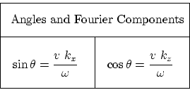
Now for the whistles, bells, and trumpets. Equating (7.8) to the real part of (7.9), physical angles and velocity are related to Fourier components. The Fourier kernel has the form of a plane wave. These relations should be memorized!

$$\vbox{\offinterlineskip \hrule \halign {&\vrule ...$$ (10)

A point in $(\omega,k_x,k_z)$-space is a plane wave. The one-dimensional Fourier kernel extracts frequencies. The multi-dimensional Fourier kernel extracts (monochromatic) plane waves.

Equally important is what comes next. Insert the angle definitions into the familiar relation $\sin^2 \theta + \cos^2 \theta = 1$. This gives a most important relationship:

$$k_x^2 + k_z^2 = { \omega^2 \over v^2 }$$ (11)

The importance of (7.11) is that it enables us to make the distinction between an arbitrary function and a chaotic function that actually is a wavefield. Imagine any function $u(t,x,z)$. Fourier transform it to $U(\omega , k_x , k_z )$. Look in the $(\omega,k_x,k_z)$-volume for any nonvanishing values of $U$. You will have a wavefield if and only if all nonvanishing $U$ have coordinates that satisfy (7.11). Even better, in practice the $(t,x)$-dependence at $z = 0$ is usually known, but the $z$-dependence is not. Then the $z$-dependence is found by assuming $U$ is a wavefield, so the $z$-dependence is inferred from (7.11).

Equation (7.11) also achieves fame as the ``dispersion relation of the scalar wave equation,'' a topic developed more fully in IEI.

Given any $f(t)$ and its Fourier transform $F(\omega)$ we can shift $f(t)$ by $t_0$ if we multiply $F(\omega)$ by $e^{i\omega t_0}$. This also works on the $z$-axis. If we were given $F(k_z)$ we could shift it from the earth surface $z = 0$ down to any $z_0$ by multiplying by $e^{ik_z z_0}$. Nobody ever gives us $F(k_z)$, but from measurements on the earth surface $z = 0$ and double Fourier transform, we can compute $F(\omega,k_x)$. If we assert/assume that we have measured a wavefield, then we have $k_z^2 = \omega^2/v^2 - k_x^2$, so knowing $F(\omega,k_x)$ means we know $F(k_z)$. Actually, we know $F(k_z,k_x)$. Technically, we also know $F(k_z,\omega)$, but we are not going to use it in this book.

We are almost ready to extrapolate waves from the surface into the earth but we need to know one more thing -- which square root do we take for $k_z$? That choice amounts to the assumption/assertion of upcoming or downgoing waves. With the exploding reflector model we have no downgoing waves. A more correct analysis has two downgoing waves to think about: First is the spherical wave expanding about the shot. Second arises when upcoming waves hit the surface and reflect back down. The study of multiple reflections requires these waves.

Downward continuation