Field recording geometry

RECORDING GEOMETRY

Along the horizontal $x$-axis we define two points, $s$, where the source (or shot or sender) is located, and $g$, where the geophone (or hydrophone or microphone) is located. Then, define the midpoint $y$ between the shot and geophone, and define $h$ to be half the horizontal offset between the shot and geophone:

$$y = {g + s \over 2 }$$ (1)

$$h = {g - s \over 2 }$$ (2)

The reason for using half the offset in the equations is to simplify and symmetrize many later equations. Offset is defined with $g - s$ rather than with $s - g$ so that positive offset means waves moving in the positive $x$ direction. In the marine case, this means the ship is presumed to sail negatively along the $x$-axis. In reality the ship may go either way, and shot points may either increase or decrease as the survey proceeds. In some situations you can clarify matters by setting the field observer's shot-point numbers to negative values.

Data is defined experimentally in the space of $(s, g)$. Equations (1.1) and (1.2) represent a change of coordinates to the space of $(y, h)$. Midpoint-offset coordinates are especially useful for interpretation and data processing. Since the data is also a function of the travel time $t$, the full dataset lies in a volume. Because it is so difficult to make a satisfactory display of such a volume, what is customarily done is to display slices. The names of slices vary slightly from one company to the next. The following names seem to be well known and clearly understood:

$(y, h = 0, t)$	zero-offset section
$(y, h = h_{\rm min ,} t)$	near-trace section
$(y, h = \hbox{const} , t)$	constant-offset section
$(y, h = h_{\rm max ,} t)$	far-trace section
$(y = \hbox{const} , h, t)$	common-midpoint gather
$(s = \hbox{const} , g, t)$	field profile (or common-shot gather)
$(s, g = \hbox{const} , t)$	common-geophone gather
$(s, g, t = \hbox{const} )$	time slice
$(h, y, t = \hbox{const} )$	time slice

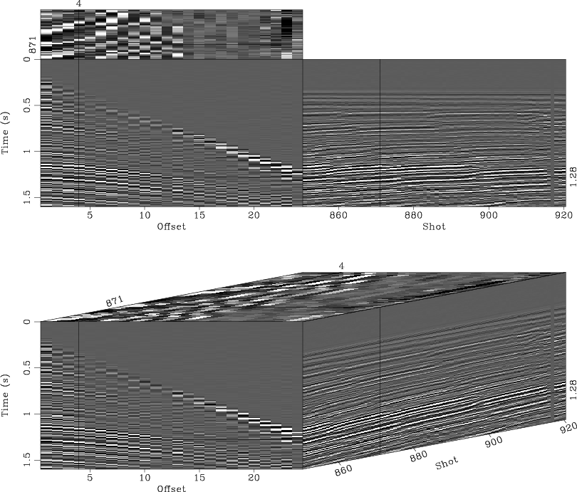
A diagram of slice names is in Figure 1.1. Figure 1.2 shows three slices from the data volume. The first mode of display is ``engineering drawing mode.'' The second mode of display is on the faces of a cube. But notice that although the data is displayed on the surface of a cube, the slices themselves are taken from the interior of the cube. The intersections of slices across one another are shown by dark lines.

sg
Figure 1. Top shows field recording of marine seismograms from a shot at location $s$ to geophones at locations labeled $g$. There is a horizontal reflecting layer to aid interpretation. The lower diagram is called a stacking diagram. (It is not a perspective drawing). Each dot in this plane depicts a possible seismogram. Think of time running out from the plane. The center geophone above (circled) records the seismogram (circled dot) that may be found in various geophysical displays. Lines in this $(s,g)$-plane are planes in the $(t,s,g)$-volume. Planes of various orientations have the names given in the text.

cube
Figure 2. Slices from within a cube of data. Top: Slices displayed as a mechanical drawing. Bottom: Same slices shown on perspective of cube faces.

A common-depth-point (CDP) gather is defined by the industry and by common usage to be the same thing as a common-midpoint (CMP) gather. But in this book a distinction will be made. A CDP gather is a CMP gather with its time axis stretched according to some velocity model, say,

$$(y=\hbox{const}, h, \sqrt{t^2 - 4h^2 /v^2 }) \quad \quad \hbox{common-depth-point gather}$$

This offset-dependent stretching makes the time axis of the gather become more like a depth axis, thus providing the D in CDP. The stretching is called normal moveout correction (NMO). Notice that as the velocity goes to infinity, the amount of stretching goes to zero.

There are basically two ways to get two-dimensional information from three-dimensional information. The most obvious is to cut out the slices defined above. A second possibility is to remove a dimension by summing over it. In practice, the offset axis is the best candidate for summation. Each CDP gather is summed over offset. The resulting sum is a single trace. Such a trace can be constructed at each midpoint. The collection of such traces, a function of midpoint and time, is called a CDP stack. Roughly speaking, a CDP stack is like a zero-offset section, but it has a less noisy appearance.

The construction of a CDP stack requires that a numerical choice be made for the moveout-correction velocity. This choice is called the stacking velocity. The stacking velocity may be simply someone's guess of the earth's velocity. Or the guess may be improved by stacking with some trial velocities to see which gives the strongest and least noisy CDP stack.

Figures 1.3 and 1.4 show typical marine and land profiles (common-shot gathers).

yc02 Figure 3. A seismic land profile. There is a gap where there are no receivers near the shot. You can see events of three different velocities. (Western Geophysical).

yc20 Figure 4. A marine profile off the Aleutian Islands. (Western Geophysical).

The land data has geophones on both sides of the source. The arrangement shown is called an uneven split spread. The energy source was a vibrator. The marine data happens to nicely illustrate two or three head waves. 1

Field recording geometry