|
|
|
|
Waves and Fourier sums |
In this book waves go down into the earth; they reflect; they come back up; and then they disappear. In reality after they come back up they reflect from the earth surface and go back down for another episode. Such waves, called multiple reflections, in real life are in some places negligible while in other places they overwhelm. Some places these multiply reflected waves can be suppressed because their RMS velocity tends to be slower because they spend more time in shallower regions. In other places this is not so. We can always think of making an earth model, using it to predict the multiply reflected waveforms, and subtracting the multiples from the data. But a serious pitfall is that we would need to have the earth model in order to find the earth model.
Fortunately, a little Fourier transform magic goes a long
way towards solving the problem.
Take a shot profile ![]() .
Fourier transform it to
.
Fourier transform it to
![]() .
For every
.
For every ![]() and
and ![]() , square this value
, square this value
![]() .
Inverse Fourier transform.
In
Figure 7
we inspect the result.
For the squared part the
.
Inverse Fourier transform.
In
Figure 7
we inspect the result.
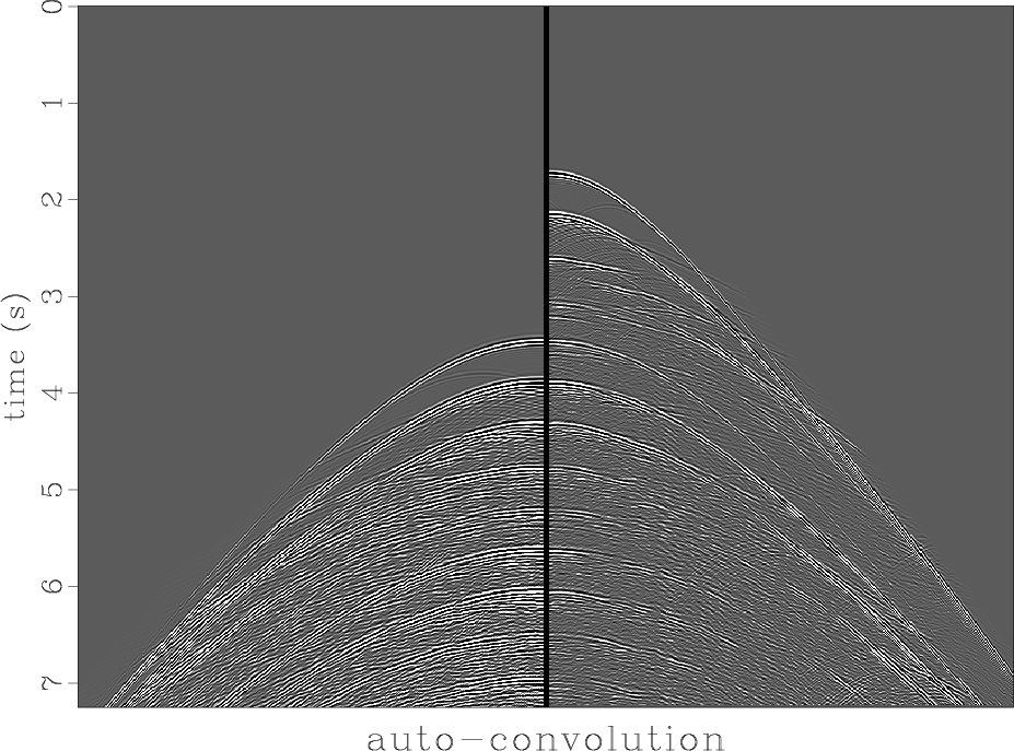
For the squared part the ![]() -axis is reversed
to facilitate comparison at zero offset.
A great many reflections on the raw data (right) carry over into the
predicted multiples (left).
If not, they are almost certainly primary reflections.
This data shows more multiples than primaries.
-axis is reversed
to facilitate comparison at zero offset.
A great many reflections on the raw data (right) carry over into the
predicted multiples (left).
If not, they are almost certainly primary reflections.
This data shows more multiples than primaries.
|
|---|
|
brad1
Figure 7. Data (right) with its FT squared (left). |
|
|
Why does this work? Why does squaring the Fourier Transform of the raw
data give us this good looking estimate of the multiple reflections?
Recall ![]() -transforms
-transforms
![]() .
A
.
A ![]() -transform is really a Fourier transform.
Take a signal that is an impulse of amplitude r at time
-transform is really a Fourier transform.
Take a signal that is an impulse of amplitude r at time ![]() .
Its
.
Its ![]() -transform is
-transform is ![]() .
The square of this
.
The square of this ![]() -transform is
-transform is ![]() ,
just what we expect of a multiple reflection --
squared amplitude and twice the travel time.
That explains vertically propagating waves.
When a ray has a horizontal component,
an additional copy of the ray doubles the horizontal distance traveled.
Remember what squaring a Fourier transformation does - a convolution.
Here the convolution is over both
,
just what we expect of a multiple reflection --
squared amplitude and twice the travel time.
That explains vertically propagating waves.
When a ray has a horizontal component,
an additional copy of the ray doubles the horizontal distance traveled.
Remember what squaring a Fourier transformation does - a convolution.
Here the convolution is over both ![]() and
and ![]() .
Every bit of the echo upon reaching the earth surface
turns around and pretends it is a new little shot.
Mathematically, every point in the upcoming wave
.
Every bit of the echo upon reaching the earth surface
turns around and pretends it is a new little shot.
Mathematically, every point in the upcoming wave ![]() launches a replica
of
launches a replica
of ![]() shifted in both time and space - an autoconvolution.
shifted in both time and space - an autoconvolution.
In reality, multiple reflections offer a considerable number of challenges that I'm not mentioning. The point here is just that FT is a good tool to have.
|
|
|
|
Waves and Fourier sums |