Zero-offset migration

Fast Kirchhoff code

Subroutine kirchslow() can easily be speeded by a factor that is commonly more than 30. The philosopy of this book is to avoid minor optimizations, but a factor of 30 really is significant, and the analysis required for the speed up is also interesting. Much of the inefficiency of kirchslow() arises when $x_{\max} \gg v t_{\max}$ because then many values of $t$ are computed beyond $t_{\max}$. To avoid this, we notice that for fixed offset (ix-iy) and variable depth iz, as depth increases, time it eventually goes beyond the bottom of the mesh and, as soon as this happens, it will continue to happen for all larger values of iz. Thus we can break out of the iz loop the first time we go off the mesh to avoid computing anything beyond as shown in subroutine kirchfast(). (Some quality compromises, limiting the aperture or the dip, also yield speedup, but we avoid those.) Another big speedup arises from reusing square roots. Since the square root depends only on offset and depth, once computed it can be used for all ix. Finally, these changes of variables have left us with more complicated side boundaries, but once we work these out, the inner loops can be devoid of tests and in kirchfast() they are in a form that is highly optimizable by many compilers.

user/gee/kirchfast.c

    for (ib= -nx; ib <= nx; ib++) { /* offset */
        for (iz=1; iz < nt; iz++) { /* travel-time depth */
	    z = t0 + dt * iz;
	    t = hypotf(z,ib*dx/vrms[iz]);
	    it = 0.5 + (t - t0) / dt;
	    if( it > nt ) break;

	    amp = (z / t)  *  sqrtf( nt*dt / t );
	    for (ix=SF_MAX(0,-ib); ix<SF_MIN(nx,nx-ib); ix++) {
		id = it + (ix+ib)*nt;
		im = iz + ix*nt;

		if( adj) modl[im] += data[id]*amp;
		else     data[id] += modl[im]*amp;
	    }
	}
    }

Originally the two Kirchhoff programs produced identical output, but finally I could not resist adding an important feature to the fast program, scale factors $z/t=\cos\theta$ and $1/\sqrt{t}$ that are described elsewhere. The fast program allows for velocity variation with depth. When velocity varies laterally the story becomes much more complicated.

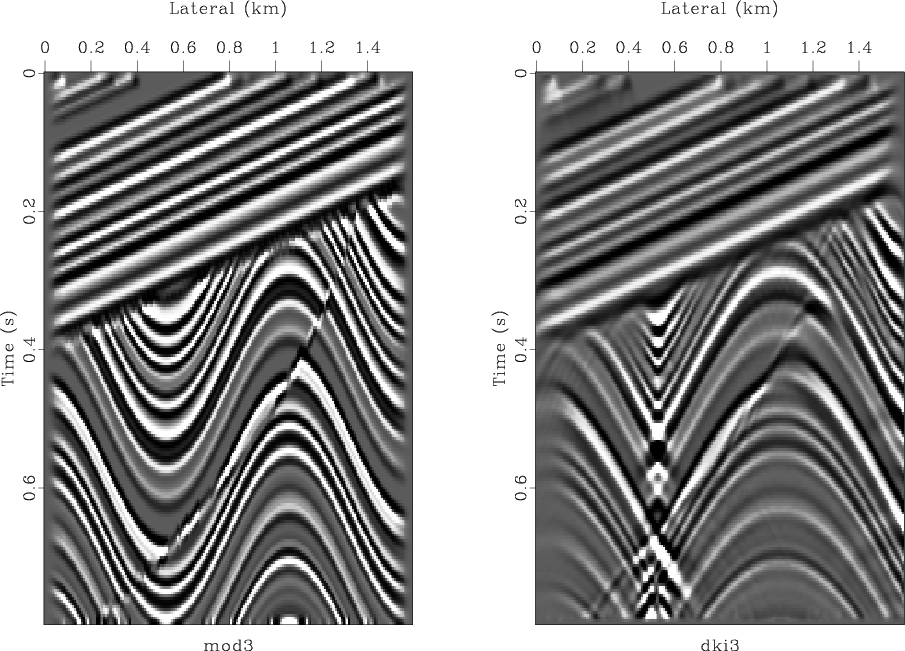
Figure 5.7 shows an example. The model includes dipping beds, syncline, anticline, fault, unconformity, and buried focus. The result is as expected with a ``bow tie'' at the buried focus. On a video screen, I can see hyperbolic events originating from the unconformity and the fault. At the right edge are a few faint edge artifacts. We could have reduced or eliminated these edge artifacts if we had extended the model to the sides with some empty space.

kfgood
Figure 7. Left is the model. Right is diffraction to synthetic data.

Zero-offset migration