|
|
|
|
Interferometric imaging condition for wave-equation migration |


|
|---|
|
parray,aarray
Figure 1. Zero-offset seismic experiment sketch (a) and multi-offset seismic experiment sketch (b). Coordinates |
|
|
Mathematically, we can represent the wavefield ![]() reconstructed at
coordinates
reconstructed at
coordinates
![]() from data
from data ![]() recorded at coordinates
recorded at coordinates
![]() as a
temporal convolution of the recorded trace with the Green's function
as a
temporal convolution of the recorded trace with the Green's function
![]() connecting the two points:
connecting the two points:
The Green's function used in the procedure described by equation 1 can be implemented in different ways. For our purposes, the actual method used for computing Green's functions is not relevant. Any procedure can be used, although different procedures will be appropriate in different situations, with different cost of implementation. We assume that a satisfactory procedure exists and is appropriate for the respective velocity models used for the simulations. In our examples, we compute Green's functions with time-domain finite-difference solutions to the acoustic wave-equation, similar to reverse-time migration (Baysal et al., 1983).


|
|---|
|
pvo,xm
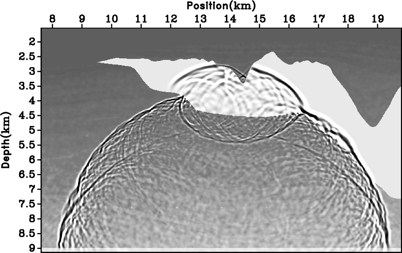
Figure 2. Velocity model (a) and imaging target located around |
|
|


|
|---|
|
pwo-0,pwv-0,pwo-7,pwv-7,pdo,pdv
Figure 3. Seismic snapshots of acoustic wavefields simulated in the background velocity model (a)-(c), and in the random velocity model (b)-(d). Data recorded at the surface from simulation in the background velocity model (e) and from the simulation in the random velocity model (f). |
|
|
Consider the velocity model depicted in Figure 2(a) and the
imaging target depicted in Figure 2(b). We assume that the model
with random fluctuations (Figure 3(b)) represents the real
subsurface velocity and use this model to simulate data. We consider
the background model (Figure 3(a)) to represent the migration
velocity and use this model to migrate the data simulated in the
random model. We consider one source located in the subsurface at
coordinates ![]() km and
km and ![]() km, and receivers located close to
the top of the model at discrete horizontal positions and depth
km, and receivers located close to
the top of the model at discrete horizontal positions and depth
![]() km. Figure 3(c)-3(d) show snapshots of
the simulated wavefields at a later time. The panels on the left
correspond to modeling in the background model, while the panels on
the right correspond to modeling in the random model.
km. Figure 3(c)-3(d) show snapshots of
the simulated wavefields at a later time. The panels on the left
correspond to modeling in the background model, while the panels on
the right correspond to modeling in the random model.
Figure 3(f) shows the data recorded on the surface. The direct wavefield arrival from the seismic source is easily identified in the data, although the wavefronts are distorted by the random perturbations in the medium. For comparison, Figure 3(e) shows data simulated in the background model, which do not show random fluctuations.
Conventional imaging using the procedure described above implicitly states that data generated in the random model, Figure 3(b), are processed as if they were generated in the background model, Figure 3(a). Thus, the random phase variations in the data are not properly compensated during the imaging procedure causing artifacts in the image. Figure 6(b) shows the image obtained by migrating data from Figure 3(f) using the model from Figure 3(a). For comparison, Figure 6(a) shows the image obtained by migrating the data from Figure 3(e) using the same model from Figure 3(a).
Ignoring aperture effects, the artifacts observed in the images are caused only by the fact that the velocity models used for modeling and migration are not the same. Small artifacts caused by truncation of the data on the acquisition surface can also be observed, but those artifacts are well-known (i.e. truncation butterflies) and are not the subject of our analysis. In this example, the wavefield reconstruction procedure is the same for both modeling and migration (i.e. time-domain finite-difference solution to the acoustic wave-equation), thus it is not causing artifacts in the image. We can conclude that the migration artifacts are simply due to the phase errors between the Green's functions used for modeling (with the random velocity) and the Green's functions used for migration (with the background velocity). The main challenge for imaging in media with random variations is to design procedures that attenuate the random phase delays introduced in the recorded data by the unknown variations of the medium without damaging the real reflections present in the data.
The random phase fluctuations observed in recorded data (Figure 3(f)) are preserved during wavefield reconstruction using the background velocity model. We can observe the randomness in the extrapolated wavefields in two ways, by reconstructing wavefields using individual data traces separately, or by reconstructing wavefields using all data traces at once.
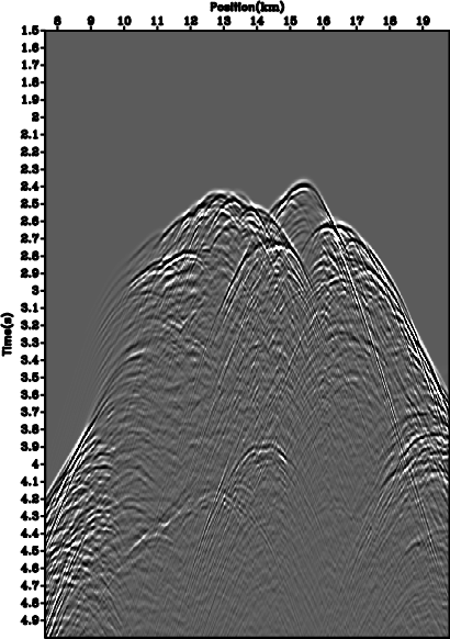
The first option is to reconstruct the seismic wavefield at all image
locations
![]() from individual receiver positions on the
surface. Of course, this is not conventionally done in reverse-time
imaging, but we describe this concept just for illustration purposes.
Figure 4(a) shows the wavefield reconstructed separately from
individual data traces depicted in Figure 3(f) using the
background model depicted in Figure 3(b). In Figure 4(a),
the horizontal axis corresponds to receiver positions on the surface,
i.e. coordinates
from individual receiver positions on the
surface. Of course, this is not conventionally done in reverse-time
imaging, but we describe this concept just for illustration purposes.
Figure 4(a) shows the wavefield reconstructed separately from
individual data traces depicted in Figure 3(f) using the
background model depicted in Figure 3(b). In Figure 4(a),
the horizontal axis corresponds to receiver positions on the surface,
i.e. coordinates
![]() , and the vertical axis represents time.
According to the notations used in this paper, Figure 4(a) shows
the wavefield
, and the vertical axis represents time.
According to the notations used in this paper, Figure 4(a) shows
the wavefield
![]() reconstructed to a particular image
coordinate
reconstructed to a particular image
coordinate
![]() from separate traces located on the surface at
coordinates
from separate traces located on the surface at
coordinates
![]() . A similar plot can be constructed for all other
image locations. Ideally, the reconstructed wavefield should line-up
at time
. A similar plot can be constructed for all other
image locations. Ideally, the reconstructed wavefield should line-up
at time ![]() , but this is not what we observe in this figure,
indicating that the input data contain random phase delays that are
not compensated during wavefield reconstruction using the background
velocity.
, but this is not what we observe in this figure,
indicating that the input data contain random phase delays that are
not compensated during wavefield reconstruction using the background
velocity.
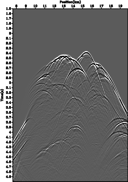
The second option is to reconstruct the seismic wavefield at all image
locations
![]() from all receiver positions on the surface at
once. This is a conventional procedure for reverse-time imaging.
Figure 5(a) shows the wavefield reconstructed from all
data traces depicted in Figure 3(f) using the background model
depicted in Figure 3(b). In Figure 5(a), the vertical and
horizontal axes correspond to depth and horizontal positions around
the source, i.e. coordinates
from all receiver positions on the surface at
once. This is a conventional procedure for reverse-time imaging.
Figure 5(a) shows the wavefield reconstructed from all
data traces depicted in Figure 3(f) using the background model
depicted in Figure 3(b). In Figure 5(a), the vertical and
horizontal axes correspond to depth and horizontal positions around
the source, i.e. coordinates
![]() , and the third cube axis represents
time. According to the notations used in this paper, Figure 5(a)
corresponds to wavefield
, and the third cube axis represents
time. According to the notations used in this paper, Figure 5(a)
corresponds to wavefield
![]() reconstructed from data at all
receiver coordinates
reconstructed from data at all
receiver coordinates
![]() to image coordinates
to image coordinates
![]() . The
reconstructed wavefield does not focus completely at the image
coordinate and time
. The
reconstructed wavefield does not focus completely at the image
coordinate and time ![]() indicating that the input data contains
random phase delays that are not compensated during wavefield
reconstruction using the background velocity.
indicating that the input data contains
random phase delays that are not compensated during wavefield
reconstruction using the background velocity.
|
|
|
|
Interferometric imaging condition for wave-equation migration |