|
|
|
|
Elastic wave-mode separation for TTI media |
To obtain the polarization vectors for P and S modes in the symmetry
planes of TTI media, one needs to solve for the Christoffel equation 3
with
| (8) | |||
| (9) | |||
| (10) |
In anisotropic media, ![]() generally deviates from the wave vector
direction
generally deviates from the wave vector
direction
![]() , where
, where ![]() is the angular
frequency,
is the angular
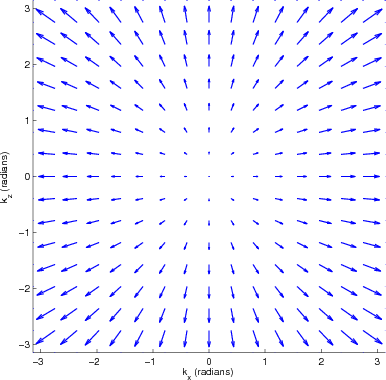
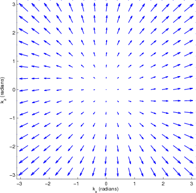
frequency, ![]() is the phase vector. Figures 1(a) and fig:TTIpolar
show the P-mode polarization in the wavenumber domain for a VTI medium
and a TTI medium with a 30
is the phase vector. Figures 1(a) and fig:TTIpolar
show the P-mode polarization in the wavenumber domain for a VTI medium
and a TTI medium with a 30![]() tilt angle, respectively. The
polarization vectors for the VTI medium deviate from radial
directions, which represent the isotropic polarization vectors
tilt angle, respectively. The
polarization vectors for the VTI medium deviate from radial
directions, which represent the isotropic polarization vectors
![]() . The polarization vectors of the TTI medium are rotated
30
. The polarization vectors of the TTI medium are rotated
30![]() about the origin from the vectors of the VTI medium.
about the origin from the vectors of the VTI medium.
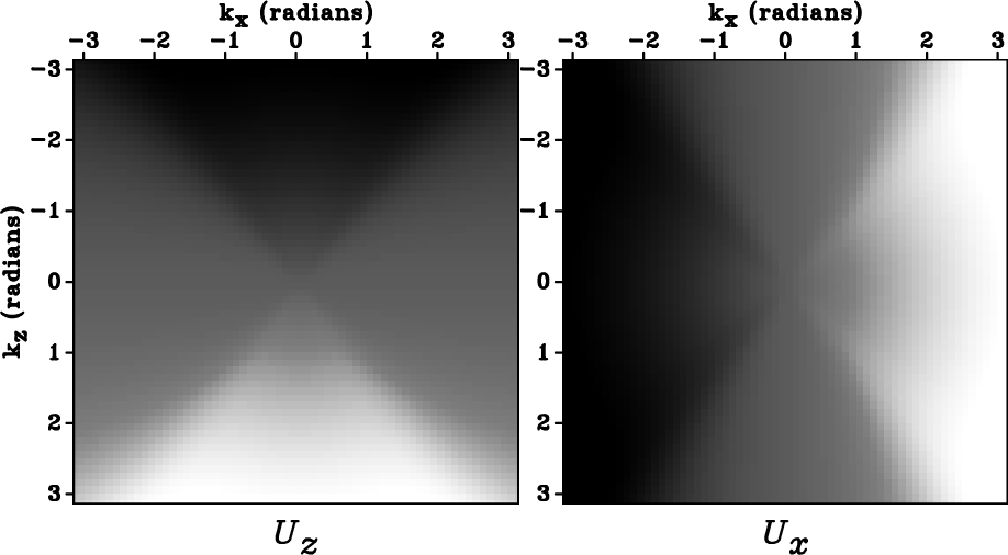
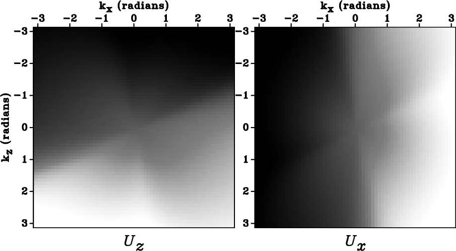
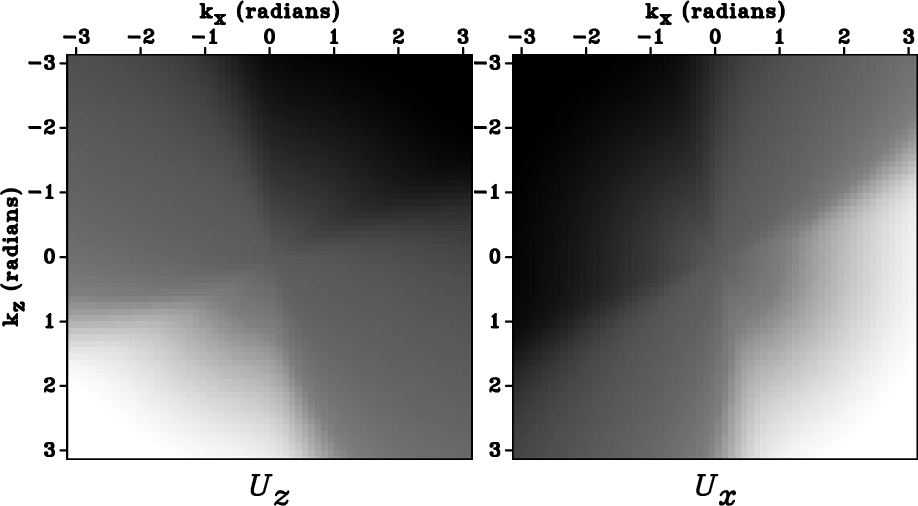
Figures ![]() and fig:dK_notaper_TTI show the components
of the P-wave polarization of a VTI medium and a TTI medium with a
30
and fig:dK_notaper_TTI show the components
of the P-wave polarization of a VTI medium and a TTI medium with a
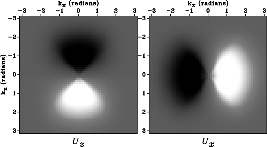
30![]() tilt angle, respectively. Figure
tilt angle, respectively. Figure ![]() shows
that the polarization vectors in Figure
shows
that the polarization vectors in Figure ![]() rotated to the
symmetry axis and its orthogonal direction of the TTI
medium. Comparing Figures
rotated to the
symmetry axis and its orthogonal direction of the TTI
medium. Comparing Figures ![]() and fig:dK_notaper_rot_TTI,
we see that within the circle of radius
and fig:dK_notaper_rot_TTI,
we see that within the circle of radius ![]() radians, the components of this
TTI medium are rotated 30
radians, the components of this
TTI medium are rotated 30![]() from those of the VTI
medium. However, note that the
from those of the VTI
medium. However, note that the ![]() and
and ![]() components of the
polarization vectors for the VTI medium (Figure
components of the
polarization vectors for the VTI medium (Figure ![]() ) are
symmetric with respect to the
) are
symmetric with respect to the ![]() and
and ![]() axes, respectively; in
contrast, the vectors of the TTI medium (Figure
axes, respectively; in
contrast, the vectors of the TTI medium (Figure ![]() ) are
not symmetric because of the non-alignment of the TTI symmetry with
the Cartesian coordinates.
) are
not symmetric because of the non-alignment of the TTI symmetry with
the Cartesian coordinates.
To maintain continuity at the negative and positive Nyquist
wavenumbers for Fourier transform to obtain space-domain filters,
i.e. at
![]() radians, one needs to apply tapers to the vector
components. For VTI media, a taper corresponding to the
function (Yan and Sava, 2009)
radians, one needs to apply tapers to the vector
components. For VTI media, a taper corresponding to the
function (Yan and Sava, 2009)
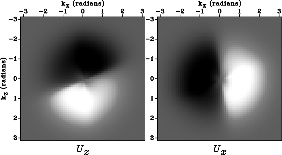
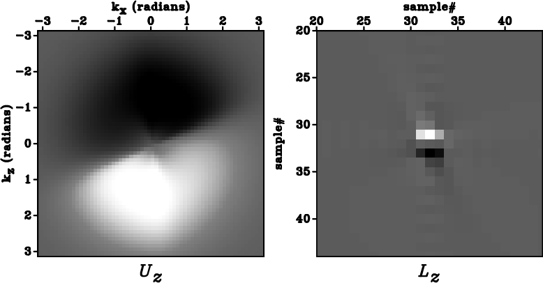
For TTI media, due to the asymmetry of the Fourier domain derivatives
(Figure ![]() ), one needs to apply a rotational symmetric
taper to the polarization vector components to obtain continuity
across Nyquist wavenumbers. A simple Gaussian taper
), one needs to apply a rotational symmetric
taper to the polarization vector components to obtain continuity
across Nyquist wavenumbers. A simple Gaussian taper
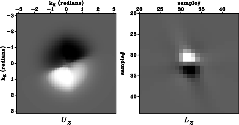
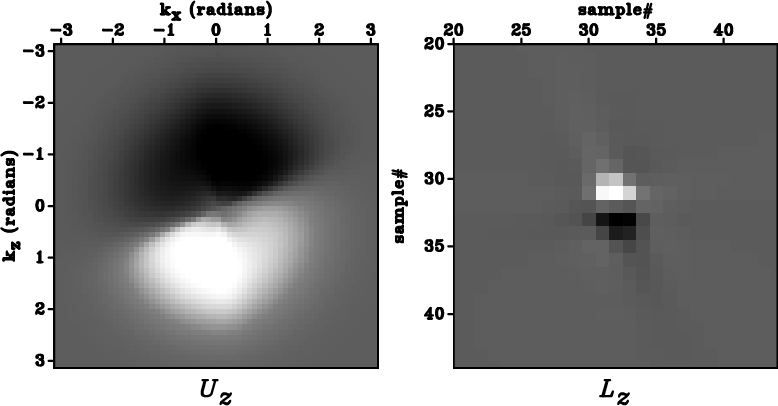
The value of ![]() determines the size of the operators in the
space domain and also affects the frequency content of the separated
wave-modes. For example, Figure 5 shows the component
determines the size of the operators in the
space domain and also affects the frequency content of the separated
wave-modes. For example, Figure 5 shows the component ![]() and operator
and operator ![]() for
for ![]() values of
values of ![]() ,
, ![]() , and
, and ![]() radians. A larger value of
radians. A larger value of ![]() results in more concentrated
operators in the space domain and better preserved frequency of the
separated wave-modes. However, one needs to ensure that the function
results in more concentrated
operators in the space domain and better preserved frequency of the
separated wave-modes. However, one needs to ensure that the function
![]() at
at
![]() radians is small enough to assume
continuity of the value function across Nyquist wavenumbers. When one
chooses
radians is small enough to assume
continuity of the value function across Nyquist wavenumbers. When one
chooses ![]() radian, the TTI components can be safely assumed to
be continuous across the Nyquist wavenumbers.
radian, the TTI components can be safely assumed to
be continuous across the Nyquist wavenumbers.
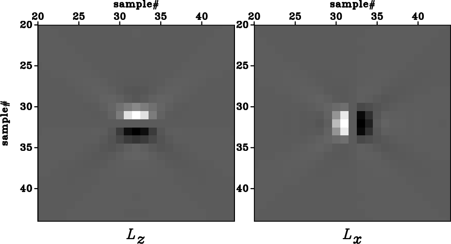
For heterogeneous models, I can pre-compute the polarization vectors
at each grid point as a function of the
![]() ratio, the
Thomsen parameters
ratio, the
Thomsen parameters ![]() and
and ![]() , and tilt angle
, and tilt angle ![]() . I
then transform the tapered polarization vector components to the space
domain to obtain the spatially-varying separators
. I
then transform the tapered polarization vector components to the space
domain to obtain the spatially-varying separators ![]() and
and ![]() . The
separators for the entire model are stored and used to separate P- and
S-modes from reconstructed elastic wavefields at different time
steps. Thus, wavefield separation in TI media can be achieved simply
by non-stationary filtering with spatially varying operators. I
assume that the medium parameters vary slowly in space and that they
are locally homogeneous. For complex media, the localized operators
behave similarly to the long finite difference operators used for
finite difference modeling at locations where medium parameters change
rapidly.
. The
separators for the entire model are stored and used to separate P- and
S-modes from reconstructed elastic wavefields at different time
steps. Thus, wavefield separation in TI media can be achieved simply
by non-stationary filtering with spatially varying operators. I
assume that the medium parameters vary slowly in space and that they
are locally homogeneous. For complex media, the localized operators
behave similarly to the long finite difference operators used for
finite difference modeling at locations where medium parameters change
rapidly.
|
|---|
|
VTIpolar,TTIpolar
Figure 1. The polarization vectors of P-mode as a function of normalized wavenumbers |
|
|
|
|---|
|
dK-notaper-VTI,dK-notaper-TTI,dK-notaper-rot-TTI
Figure 2. The |
|
|

|
|---|
|
dK-VTI,dK-TTI,dK-rot-TTI
Figure 3. The wavenumber-domain vectors in Figure 2 are tapered by the function in equation 12 to avoid Nyquist discontinuity. Panel (a) corresponds to Figure 2(a), panel (b) corresponds to Figure 2(b), and panel (c) corresponds to Figure 2(c). |
|
|
|
|---|
|
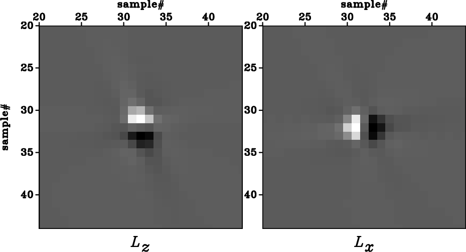
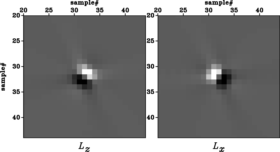
dX-VTI,dX-TTI,dX-rot-TTI
Figure 4. The space-domain wave-mode separators for the medium shown in Figure 1. They are the Fourier transformation of the polarization vectors shown in Figure 3. Panel (a) corresponds to Figure 3(a), panel (b) corresponds to Figure 3(b), and panel (c) corresponds to Figure 3(c). The zoomed views show |
|
|
|
|---|
|
dzKX-sig0-TTI,dzKX-sig1-TTI,dzKX-sig2-TTI
Figure 5. Panels (a)-(c) correspond to component |
|
|
|
|
|
|
Elastic wave-mode separation for TTI media |
![$\displaystyle g({\bf k})=C exp\left [-\frac{\left\vert{\bf k}\right\vert^2}{2\sigma^2}\right]$](img77.png)