 |
 |
 |
 | Model fitting by least squares |  |
![[pdf]](icons/pdf.png) |
Next: Routine for one step
Up: KRYLOV SUBSPACE ITERATIVE METHODS
Previous: The magical property of
Fourier-transformed variables are often capitalized.
This convention is helpful here,
so in this subsection only,
we capitalize vectors transformed by the  matrix.
As everywhere, a matrix, such as ,
is printed in boldface type
but in this subsection,
vectors are not printed in boldface.
Thus, we define the solution, the solution step
(from one iteration to the next),
and the gradient by:
matrix.
As everywhere, a matrix, such as ,
is printed in boldface type
but in this subsection,
vectors are not printed in boldface.
Thus, we define the solution, the solution step
(from one iteration to the next),
and the gradient by:
A linear combination in solution space,
say  , corresponds to
  in the conjugate space, the data space,
because
in the conjugate space, the data space,
because
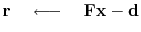
 .
According to equation
(51),
the residual is the modeled data minus the observed data.
.
According to equation
(51),
the residual is the modeled data minus the observed data.
 |
(69) |
The solution  is obtained by a succession of steps
  , say:
 |
(70) |
The last stage of each iteration is to update the solution and the residual:
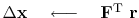
The gradient vector  is a vector with the same number
of components as the solution vector .
A vector with this number of components is:
is a vector with the same number
of components as the solution vector .
A vector with this number of components is:
The gradient in the transformed space is  ,
also known as the conjugate gradient.
,
also known as the conjugate gradient.
What is our solution update
 ?
It is some unknown amount
?
It is some unknown amount  of the gradient
  plus
another unknown amount
plus
another unknown amount  of the previous step
  .
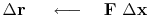
Likewise in residual space.
.
Likewise in residual space.
The minimization (56) is now generalized
to scan not only in a line with ,
but simultaneously another line with .
The combination of the two lines is a plane.
We now set out to find the location in this plane that minimizes the quadratic  .
.
 |
(77) |
The minimum is found at
 and
and
 , namely,
![\begin{displaymath}
-\ \
\left[
\begin{array}{c}
(G\cdot R) \\
(S\cdot R) \...
...eft[
\begin{array}{c}
\alpha \\
\beta \end{array} \right]
\end{displaymath}](img320.png) |
(80) |
Equation
(81)
is a set of two equations for and .
Recall the inverse of a  matrix, equation
(111)
and get:
matrix, equation
(111)
and get:
![\begin{displaymath}
\left[
\begin{array}{c}
\alpha \\
\beta \end{array} \rig...
...egin{array}{c}
(G\cdot R) \\
(S\cdot R) \end{array} \right]
\end{displaymath}](img321.png) |
(81) |
The many applications in this book all need to
find and with (81), and then
update the solution with (71) and
update the residual with (72).
Thus, we package these activities in a subroutine
named cgstep().
To use that subroutine, we have a computation template
with
repetitive work done by subroutine cgstep().
This template (or pseudocode) for minimizing the residual
 by the conjugate-direction method is:
iterate {


}
where
the subroutine cgstep()
remembers the previous iteration and
works out the step size and adds in
the proper proportion of the
 of
the previous step.
of
the previous step.
|
|
|
|
| Model fitting by least squares | |
|
Next: Routine for one step
Up: KRYLOV SUBSPACE ITERATIVE METHODS
Previous: The magical property of
2014-12-01