|
|
|
|
Model fitting by least squares |
iterate {
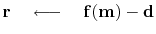
Define  .
.
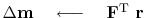

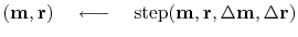
}
A formal theory for the optimization exists, but we are not using it here. The assumption we make is that the step size is small, so that familiar line-search and plane-search approximations can succeed in reducing the residual. Unfortunately, this assumption is not reliable. What we should do is test that the residual really does decrease, and if it does not, we should revert to smaller step size. Perhaps, we should test an incremental variation on the status quo: where inside solver, we check to see if the residual diminished in the previous step; and if it did not, restart the iteration (choose the current step to be steepest descent instead of CD).
Experience shows that nonlinear applications have many pitfalls.
Start with a linear problem,
add a minor physical improvement or abnormal noise,
and the problem becomes nonlinear and probably has another solution
far from anything reasonable.
When solving such a nonlinear problem,
we cannot arbitrarily begin from zero, as we do with linear problems.
We must choose a reasonable starting guess.
Chapter ![]() on the topic of regularization
offers an additional way to reduce the dangers of nonlinearity.
on the topic of regularization
offers an additional way to reduce the dangers of nonlinearity.
|
|
|
|
Model fitting by least squares |