Homework 4

Shaping regularization

For the shaping regularization approach, we are going to try the simple iteration

$$\mathbf{m}_{n+1} = \mathbf{S}_m\left[\mathbf{m}_{n} + \tilde{\mathbf{m}} - \mathbf{B F m}_n\right]\;,$$ (10)

where the forward operator $\mathbf{F}$ is bilinear interpolation, the backward operator $\mathbf{B}$ is interpolation by Delaunay triangulation, and the model shaping operator $\mathbf{S}_m$ is triangle smoothing.

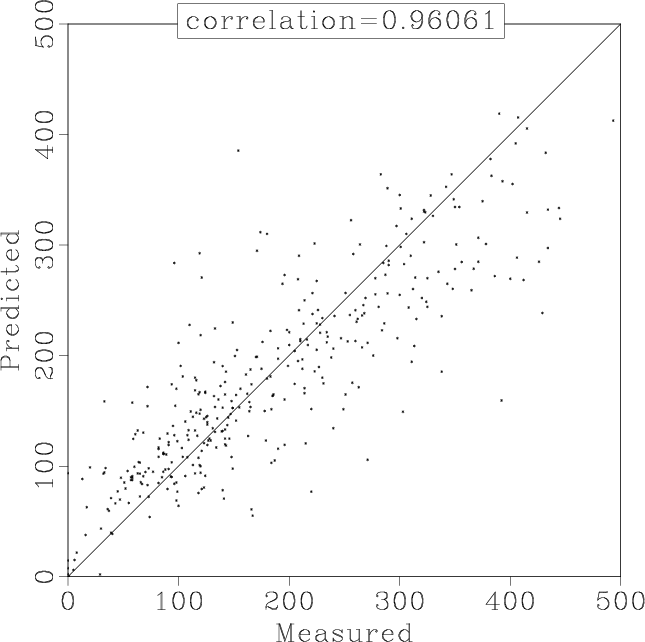
Figure 12 shows the interpolation result using 10 shaping iterations. The corresponding correlation analysis is shown in Figure 13.

shaping Figure 12. Rainfall data interpolated using shaping regularization.

shaping10-pred Figure 13. Correlation between interpolated and true data values for shaping regularization with 10 iterations.

Your task:

1. Change directory to hw4/rain
2. Run

   scons view
   

   to reproduce the figures on your screen.
3. Modify the SConstruct file to accomplish the following tasks:
   1. Find out the number of conjugate-gradient iterations needed for the gradient regularization method to achieve a result comparable with the preconditioning method.
   2. Find out the number of iterations (10) needed for the shaping regularization method to achieve a result comparable with the preconditioning method.
4. What can you conclude about the four methods used in this comparison?
5. EXTRA CREDIT Participate in the Spatial Interpolation Contest. Find and implement a method that would provide a better interpolation of the missing values than either of the methods we tried so far. You can change any of the parameters in the existing methods or write your own program but you can use only the 100 original data points as input.

/* Data regulatization by inverse interpolation. */
#include <rsf.h>

static void lint (float x, int n, float* w) 
/*< linear interpolation>*/
{
    w[0] = 1.0f - x;
    w[1] = x;
}

static void regrid( int dim         /* dimensions */, 
		    const int* nold /* old size [dim] */, 
		    const int* nnew /* new size [dim] */, 
		    sf_filter aa    /* filter */) 
/*< change data size >*/
{
    int i, h0, h1, h, ii[SF_MAX_DIM];

    for (i=0; i < dim; i++) {
	ii[i] = nold[i]/2-1;
    }
  
    h0 = sf_cart2line( dim, nold, ii); 
    h1 = sf_cart2line( dim, nnew, ii); 
    for (i=0; i < aa->nh; i++) { 
	h = aa->lag[i] + h0;
	sf_line2cart( dim, nold, h, ii);
	aa->lag[i] = sf_cart2line( dim, nnew, ii) - h1;
    }
}

int main (int argc, char* argv[])
{
    int id, nd, nm, nx, ny, na, ia, niter, three, n[2], m[2];
    float *mm, *dd, **xy;
    float x0, y0, dx, dy, a0, eps;
    char *lagfile;
    bool prec;
    sf_filter aa;
    sf_file in, out, flt, lag;

    sf_init (argc,argv);
    in = sf_input("in");
    out = sf_output("out");

    /* read data */

    if (SF_FLOAT != sf_gettype(in)) sf_error("Need float");
    if (!sf_histint(in,"n1",&three) || 3 != three) 
	sf_error("Need n1=3 in in");
    if (!sf_histint(in,"n2",&nd)) sf_error("Need n2=");

    xy = sf_floatalloc2(3,nd);
    sf_floatread(xy[0],3*nd,in);

    dd = sf_floatalloc(nd);
    for (id=0; id < nd; id++) dd[id] = xy[id][2];

    /* create model */

    if (!sf_getint ("nx",&nx)) sf_error("Need nx=");
    if (!sf_getint ("ny",&ny)) sf_error("Need ny=");
    /* Number of bins */

    sf_putint(out,"n1",nx);
    sf_putint(out,"n2",ny);

    if (!sf_getfloat("x0",&x0)) sf_error("Need x0=");
    if (!sf_getfloat("y0",&y0)) sf_error("Need y0=");
    /* grid origin */

    sf_putfloat (out,"o1",x0);
    sf_putfloat (out,"o2",y0);

    if (!sf_getfloat("dx",&dx)) sf_error("Need dx=");
    if (!sf_getfloat("dy",&dy)) sf_error("Need dy=");
    /* grid sampling */

    sf_putfloat (out,"d1",dx);
    sf_putfloat (out,"d2",dy);
 
    nm = nx*ny;
    mm = sf_floatalloc(nm);

    sf_int2_init (xy, x0,y0, dx,dy, nx,ny, lint, 2, nd);

    /* read filter */
    flt = sf_input("filt");

    if (NULL == (lagfile = sf_histstring(flt,"lag"))) 
	sf_error("Need lag= in filt");
    lag = sf_input(lagfile);

    n[0] = nx;
    n[1] = ny;
    if (!sf_histints (lag,"n",m,2)) {
	m[0] = nx;
	m[1] = ny;
    }

    if (!sf_histint(flt,"n1",&na)) sf_error("No n1= in filt");
    aa = sf_allocatehelix (na);

    if (!sf_histfloat(flt,"a0",&a0)) a0=1.;
    sf_floatread (aa->flt,na,flt);

    for( ia=0; ia < na; ia++) {
	aa->flt[ia] /= a0;
    }
	
    sf_intread(aa->lag,na,lag);
    regrid (2, m, n, aa);

    if (!sf_getbool("prec",&prec)) prec=false;
    /* if use preconditioning */

    if (!sf_getint("niter",&niter)) niter=20;
    /* number of iterations */

    if (!sf_getfloat("eps",&eps)) eps=0.01; 
    /* regularization parameter */

    if (prec) {
	sf_polydiv_init (nm, aa);
	sf_solver_prec (sf_int2_lop, sf_cgstep, 
			sf_polydiv_lop,
			nm, nm, nd, 
			mm, dd, niter, eps, "end");
    } else {
	sf_igrad2_init (nx, ny);
	sf_solver_reg (sf_int2_lop, sf_cgstep, 
		       sf_igrad2_lop,
		       2*nm, nm, nd, 
		       mm, dd, niter, eps, "end");
    }
    
    sf_floatwrite (mm,nm,out);
    exit(0);
}

from rsf.proj import *

# Download data
Fetch(['border.hh','elevation.HH',
       'alldata.hh','obsdata.hh',
       'coord.hh','predict.hh'],'rain')

# Plot limits
box = '''
min1=-185.556 max1=193.18275
min2=-127.262 max2=127.25044
'''

# Switzerland map
#################

# Border
Flow('border','border.hh','dd form=native')

f2 = 0
def border(name,n2):
    global f2
    Flow(name,'border',
         '''
         window n2=%d f2=%d |
         dd type=complex | window
         ''' % (n2,f2))
    Plot(name,'graph wanttitle=n plotcol=6 plotfat=8 ' + box)
    f2 = f2 + n2

border('border1',338)
border('border2',234)
border('border3',717)
Plot('border','border1 border2 border3','Overlay')

# Elevation
Flow('elev','elevation.HH','dd form=native')
Plot('elev',
     '''
     igrad |
     grey title="Switzerland Elevation" transp=n yreverse=n
     wantaxis=n wantlabel=n wheretitle=t wherexlabel=b
     ''')
Result('elev','elev border','Overlay')

Flow('alldata','alldata.hh',
     'window n1=2 | dd type=complex form=native | window')
Plot('alldata',
     '''
     graph symbol=x symbolsz=4
     title="All data locations" plotcol=7
     ''' + box)
Plot('data','alldata border','Overlay')

Flow('obs','obsdata.hh',
     'window n1=2 | dd type=complex form=native | window')
Plot('obs',
     '''
     graph symbol=o symbolsz=4
     title="Observed data locations" plotcol=5
     ''' + box)
Plot('obsdata','obs border','Overlay')

Result('raindata','obsdata data','SideBySideIso')

Flow('coord','coord.hh','dd form=native')
Flow('obsdata','obsdata.hh','dd form=native')

# Triangulation
###############
Flow('trian edges','obsdata elev',
     'tri2reg pattern=${SOURCES[1]} edgeout=${TARGETS[1]}')
Plot('edges',
     '''
     graph plotcol=7 plotfat=8
     wanttitle=n wantaxis=n
     ''' + box)
Plot('trian',
     '''
     grey yreverse=n transp=n allpos=y
     color=j clip=500 title="Delaunay Triangulation"
     label1="W-E (km)" label2="N-S (km)"
     ''' + box)
Result('trian','trian edges','Overlay')

# Laplacian filter
##################

Flow('lag.asc',None,
     '''
     echo 1 100 n1=2 n=100,100 
     data_format=ascii_int in=$TARGET
     ''')
Flow('lag','lag.asc','dd form=native')

Flow('flt.asc','lag',
     '''
     echo -1 -1 a0=2 n1=2 lag=$SOURCE 
     data_format=ascii_float in=$TARGET
     ''',stdin=0)
Flow('flt','flt.asc','dd form=native')

# Spectral factorization on a helix
Flow('lapflt laplag','flt',
     'wilson eps=1e-4 lagout=${TARGETS[1]}')

def plotfilt(title):
    return '''
    grey wantaxis=n title="%s" pclip=100 
    crowd=0.85 screenratio=1
    ''' % title

# Filter impulse response
Flow('spike',None,'spike n1=15 n2=15 k1=8 k2=8')
Flow('imp0','spike flt','helicon filt=${SOURCES[1]} adj=0')
Flow('imp1','spike flt','helicon filt=${SOURCES[1]} adj=1')
Flow('imp','imp0 imp1','add ${SOURCES[1]}')
Plot('imp',plotfilt('(a) Laplacian'))

# Test factorization
Flow('fac0','imp lapflt',
     'helicon filt=${SOURCES[1]} adj=0 div=1')
Flow('fac1','imp lapflt',
     'helicon filt=${SOURCES[1]} adj=1 div=1')
Plot('fac0',plotfilt('(b) Laplacian/Factor'))
Plot('fac1',plotfilt('(c) Laplacian/Factor'))
Flow('fac','fac0 lapflt',
     'helicon filt=${SOURCES[1]} adj=1 div=1')
Plot('fac',plotfilt('(d) Laplacian/Factor/Factor'))

Result('laplace','imp fac0 fac1 fac','TwoRows',
       vppen='gridsize=5,5 xsize=11 ysize=11')

# Maximum number of iterations
#############
nmax = 100 # CHANGE ME!!!

# Inverse interpolation program
program = Program('invint.c')
invint = str(program[0])

for prec in range(2):
    iters = []
    inter = 'inter%d' % prec
    for niter in [10,nmax]:
        it = 'inter%d-%d' % (prec,niter)
        Flow(it,['obsdata',invint,'lapflt'],
             '''
             ./${SOURCES[1]} prec=%d niter=%d 
             filt=${SOURCES[2]}
             nx=376 ny=253 eps=0.01
             dx=1.00997 dy=1.00997
             x0=-185.556 y0=-127.262
             ''' % (prec,niter))
        Plot(it,
             '''
             grey scalebar=y yreverse=n transp=n allpos=y
             minval=0 maxval=525 color=j clip=500
             title="%s (%d iterations)" 
             ''' % (('Regularization',
                     'Preconditioning')[prec],niter))
        iters.append(it)
    Result(inter,iters,'SideBySideIso')

# Shaping regularization
########################
# Forward - bi-linear interpolation
# Backward - triangulation
# Shaping - triangle smoothing

# Maximum number of iterations
#############
nshape = 10 # CHANGE ME!!!

m0 = 'trian'
m = m0

# Coordinates of observed data
Flow('obscoord','obsdata','window n1=2')

ms = []
for i in range(1,nshape+1):
    mi = 'shaping%d' % i
    Flow(mi,[m,'obscoord',m0],
         '''
         extract head=${SOURCES[1]} xkey=0 ykey=1     |
         transp | cat ${SOURCES[1]} axis=1 order=2,1  |
         tri2reg pattern=${SOURCES[2]}                |
         add ${SOURCES[0]} ${SOURCES[2]} scale=-1,1,1 |
         smooth rect1=20 rect2=20 repeat=2
         ''')
    Plot(mi,
         '''
         grey scalebar=y yreverse=n transp=n allpos=y
         minval=0 maxval=525 color=j clip=500
         title="Iteration %d" 
         ''' % i)
    m = mi
    ms.append(mi)
Plot('ms',ms,'Movie',view=1)
Result('shaping',mi,'Overlay')

# Prediction comparisons
########################

Flow('predict','predict.hh','dd form=native')
Flow('norm','predict',
     'add mode=p $SOURCE | stack axis=1 norm=n')

Plot('line',None,
     '''
     math n1=2 o1=0 d1=500 output=x1 |
     graph plotcol=7 wanttitle=n wantaxis=n
     screenratio=1 min1=0 max1=500 min2=0 max2=500
     ''')

for case in ('trian','shaping%d' % nshape,
             'inter0-%d' % nmax,'inter1-%d' % nmax):
    pred = case+'-pred'
    Flow(pred,[case,'coord'],
         'extract head=${SOURCES[1]} xkey=0 ykey=1')
    Plot(pred,['predict',pred],
         '''
         cmplx ${SOURCES[1]} |
         graph symbol="*" wanttitle=n
         screenratio=1 min1=0 max1=500 min2=0 max2=500
         label1=Measured label2=Predicted
         ''')

    num = case+'-num'
    den = case+'-den'
    cor = case+'-cor'

    Flow(num,['predict',pred],
         'add mode=p ${SOURCES[1]} | stack axis=1 norm=n')
    Flow(den,pred,'add mode=p $SOURCE | stack axis=1 norm=n')
    Flow(cor+'.asc',[num,den,'norm'],
         '''
         math a1=${SOURCES[1]} a2=${SOURCES[2]}
         output="input/sqrt(a1*a2)" |
         dd form=ascii -out=$TARGET
         format="label=correlation=%7.5g"
         ''',stdout=0)
    Plot(cor,cor+'.asc',
         'box x0=5.5 y0=9 xt=0 par=$SOURCE',stdin=0)
    
    Result(pred,[pred,'line',cor],'Overlay')

End()

Homework 4