|
|
|
|
Conjugate guided gradient (CGG) method for robust inversion and its application to velocity-stack inversion |
I tested the proposed CGG method on a real data set that contains various types of noise. The data set is a shot gather from a land survey. However the trajectories of the events in the data set look "hyperbolic" enough to be tested with a hyperbolic inversion.
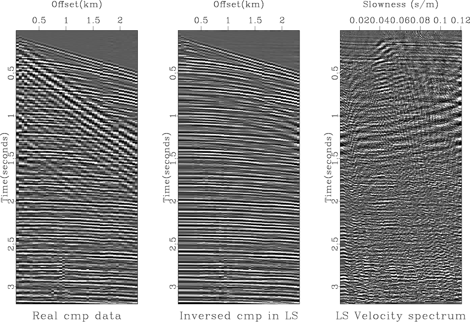
Figure 6 shows the real data set used for testing and the results, the velocity-stack (Figure 6c) and the remodeled data (Figure 6b) from it, when we used the conventional LS inversion. We can see that the real data (Figure 6a) originally contains various types of noise such as the strong ground roll, the amplitude anomalies early at near-offset and late at 0.8km offset, and the time shifts around offsets 1.6 km and 2.0 km. The conventional LS inversion generally does a good job in removing most dominant noises except some whose characteristics are somehow busty (i.e. the amplitude anomalies early at near-offset and late at 0.8km offset and the time shift around offsets 1.6 km and 2.0 km). The resultant velocity-stack panel (Figure 6c) was filled with various noises that requires some more processing if we want to perform any velocity-stack oriented processing such as velocity picking, multiple removal, and so on.
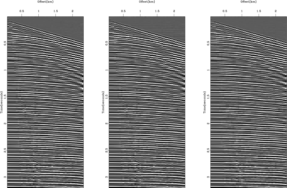
Figure 7 shows the remodeled data
from the inversion results (Figure 8) obtained using the IRLS method
with three different weighting combinations (![]() -norm residual only,
-norm residual only, ![]() -norm model only,
and
-norm model only,
and ![]() -norm residual and model together).
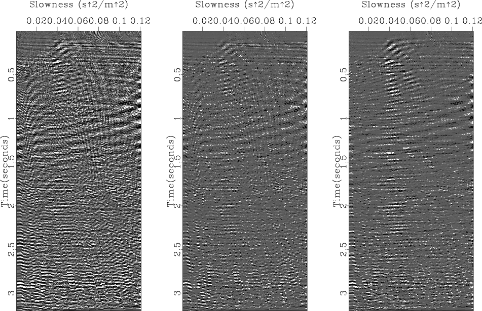
We can see that all three remodeled results show quite successful removal of most noises similarly.
The main difference among the three inversion results is the degree of parsimony
of the corresponding velocity-stacks as shown in Figure 8.
Even though the approach of the
-norm residual and model together).
We can see that all three remodeled results show quite successful removal of most noises similarly.
The main difference among the three inversion results is the degree of parsimony
of the corresponding velocity-stacks as shown in Figure 8.
Even though the approach of the ![]() -norm residual weight can reduce many noisy signals in
the velocity-stack, the result of the
-norm residual weight can reduce many noisy signals in
the velocity-stack, the result of the ![]() -norm model weight shows better parsimony of the velocity-stack.
-norm model weight shows better parsimony of the velocity-stack.
Figure 9 shows the remodeled data
from the inversion results (Figure 10)
obtained using the CGG algorithm with three different guiding types
(the residual weight only, the model weight only,
and the residual and the model weights together).
All three remodeled data (Figures 9a through 9c)
show quite similar quality as the ones obtained with IRLS method (Figure 7).
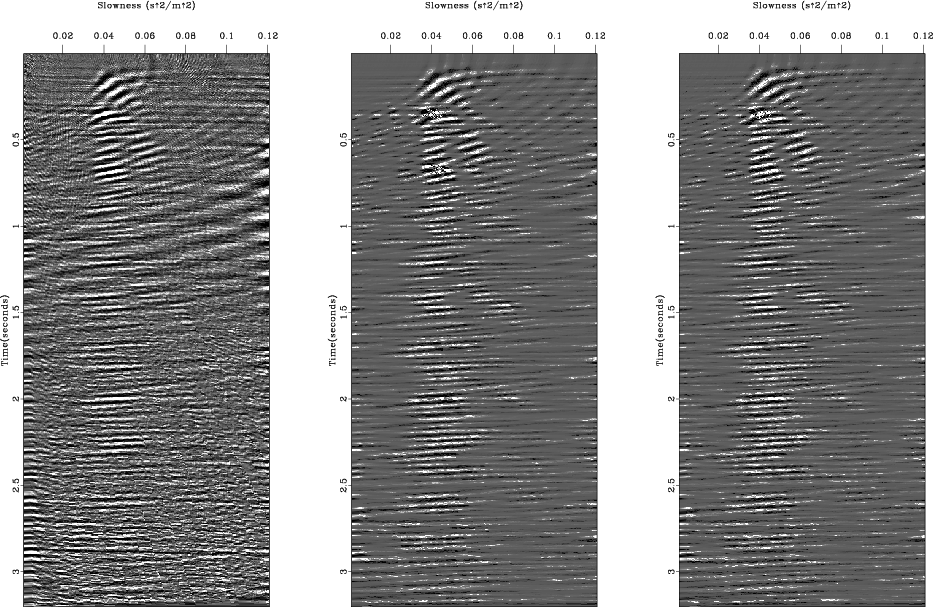
The differences in the parsimony of the velocity-stacks
among the different guiding types are also clearly shown
in the Figure 10 and they are similar to the results of IRLS method.
In the case of the guiding with the residual weight (Figure 9a)
I used the weight,
![]() to achieve
the similar quality in the noise removal as the one of the
to achieve
the similar quality in the noise removal as the one of the ![]() -norm residual minimizing IRLS method.
The exponent value
-norm residual minimizing IRLS method.
The exponent value ![]() is also decided empirically after experiments with various exponents values.
is also decided empirically after experiments with various exponents values.
|
|---|
|
wz08-L2
Figure 6. The real data set (a), the remodeled data from the inversion result (b), and the LS inversion result (c). |
|
|
|
|---|
|
wz08-IRLS
Figure 7. The remodeled data from the velocity-stack inversion results (Figure 8) of the real data (Figure 6a) using the IRLS method with different norm criteria: |
|
|
|
|---|
|
wz08-IRLS-vel
Figure 8. The velocity-stack inversion results of the real data (Figure 6a) using the IRLS method with different norm criteria: |
|
|

|
|---|
|
wz08-CGG
Figure 9. The remodeled data from the velocity-stack inversion results (Figure 10) of the real data (Figure 6a) using the CGG method with different guiding weights: the residual weight only (a), the model weight only (b), and the residual/model weights together (c). |
|
|
|
|---|
|
wz08-CGG-vel
Figure 10. The velocity-stack inversion results of the real data (Figure 6a) using the CGG method with different guiding weights: the residual weight only (a), the model weight only (b), and the residual/model weights together (c). |
|
|
In the real data example above,
the values of exponent of the weight functions in the CGG method
were decided empirically and were sometimes different from the exponents of the weights
used in the ![]() -norm IRLS method.
In the IRLS approach, the meaning of the exponent for the weight functions
can be explained either with the
-norm IRLS method.
In the IRLS approach, the meaning of the exponent for the weight functions
can be explained either with the ![]() -norm sense or
with the relative weighting for each values of the residual/model.
Even though the two explanations are closely related,
the meaning of the exponent for the weight function in the CGG method
can be explained better with the latter since it only
changes the gradient vector and doesn't minimize
-norm sense or
with the relative weighting for each values of the residual/model.
Even though the two explanations are closely related,
the meaning of the exponent for the weight function in the CGG method
can be explained better with the latter since it only
changes the gradient vector and doesn't minimize ![]() -norm.
So if we increase the value of exponent of the model weight function,
the relatively high amplitude model values get more emphasis
in fitting the model to the data.
Likewise, if we decrease the value of exponent of the residual weight function
which is a negative value, the relatively high amplitude residual values get less emphasis
in fitting the model to the data.
The optimum value of exponent or relative emphasis in the model and the residual
depends on the distribution of the values of the model/residual
and could be found empirically as performed in this paper.
The experiments performed in the paper demonstrate
that the value of exponent of weight function used for
-norm.
So if we increase the value of exponent of the model weight function,
the relatively high amplitude model values get more emphasis
in fitting the model to the data.
Likewise, if we decrease the value of exponent of the residual weight function
which is a negative value, the relatively high amplitude residual values get less emphasis
in fitting the model to the data.
The optimum value of exponent or relative emphasis in the model and the residual
depends on the distribution of the values of the model/residual
and could be found empirically as performed in this paper.
The experiments performed in the paper demonstrate
that the value of exponent of weight function used for ![]() -norm residual/model in the IRLS approach
are good choices for a start, but could be increased or decreased appropriately for each case
if any further improvement is required.
-norm residual/model in the IRLS approach
are good choices for a start, but could be increased or decreased appropriately for each case
if any further improvement is required.
|
|
|
|
Conjugate guided gradient (CGG) method for robust inversion and its application to velocity-stack inversion |