|
|
|
|
Conjugate guided gradient (CGG) method for robust inversion and its application to velocity-stack inversion |
|
|---|
|
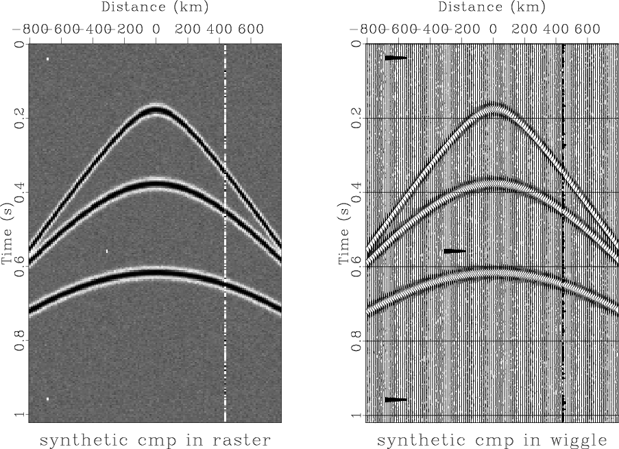
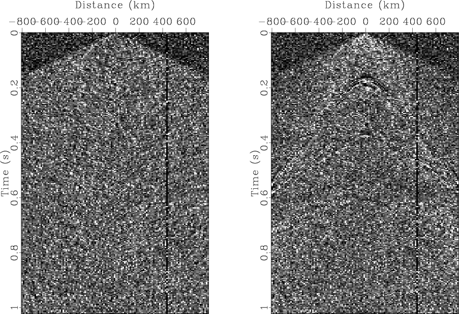
syn-data
Figure 1. Synthetic data with various types of noise in raster format (left) and in wiggle format (right). |
|
|
|
|---|
|
syn-L2
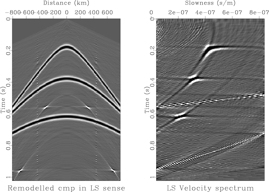
Figure 2. The remodeled synthetic data (a) from the velocity-stack (b) obtained by LS inversion using CG method for the noisy synthetic data (Figure 1). |
|
|
Figure 2 shows
the inversion result (Figure 2b) obtained using the conventional
CG algorithm for LS solution and remodeled data (Figure 2a) from it.
In the CG method, the iteration was performed 30 times
and the same number of iterations was also used for all the examples presented in this paper
(including the number of iterations in the inner loop in the case of IRLS CG method).
From Figure 2 we can clearly see the limit of ![]() -norm minimization.
In the remodeled data, the noise with Gaussian statistics was removed quite well,
but some spurious events were generated around the busty noise spikes and noisy trace.
The inversion result obtained as a velocity-stack panel
also shows many noisy values that correspond to
the noise part of the data which was not removed completely.
-norm minimization.
In the remodeled data, the noise with Gaussian statistics was removed quite well,
but some spurious events were generated around the busty noise spikes and noisy trace.
The inversion result obtained as a velocity-stack panel
also shows many noisy values that correspond to
the noise part of the data which was not removed completely.
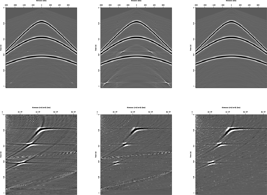
Figures 3d through 3f show the inversion results
obtained using the IRLS algorithm with ![]() -norm residual weight only,
-norm residual weight only,
![]() -norm model weight only, and
-norm model weight only, and ![]() -norm residual and model weights together, respectively.
Figures 3a through 3c show the remodeled data
from the corresponding inversion results.
From the results of
-norm residual and model weights together, respectively.
Figures 3a through 3c show the remodeled data
from the corresponding inversion results.
From the results of ![]() -norm residual weight (Figures 3a and 3d),
we can see the robustness of
-norm residual weight (Figures 3a and 3d),
we can see the robustness of ![]() -norm residual minimization for the busty noise
and the successful removal of the Gaussian noise, too.
From the results of
-norm residual minimization for the busty noise
and the successful removal of the Gaussian noise, too.
From the results of ![]() -norm model weight (Figures 3b and 3e),
we can see the improvement in the parsimony of the model compared
to the result of LS inversion (Figure 2b).
The
-norm model weight (Figures 3b and 3e),
we can see the improvement in the parsimony of the model compared
to the result of LS inversion (Figure 2b).
The ![]() -norm model weight also seems to have some effect to reduce low amplitude noise quite well
but the result shows some limit in reducing high amplitudes noises by making some spurious event around
the busty spike noises (Figure 3b).
From the results with
-norm model weight also seems to have some effect to reduce low amplitude noise quite well
but the result shows some limit in reducing high amplitudes noises by making some spurious event around
the busty spike noises (Figure 3b).
From the results with ![]() -norm residual and model weights together
(Figures 3c and 3f),
we can see that the IRLS method can achieve both goals, the robustness to the busty noises
and the parsimony of the model representation, quite well.
-norm residual and model weights together
(Figures 3c and 3f),
we can see that the IRLS method can achieve both goals, the robustness to the busty noises
and the parsimony of the model representation, quite well.
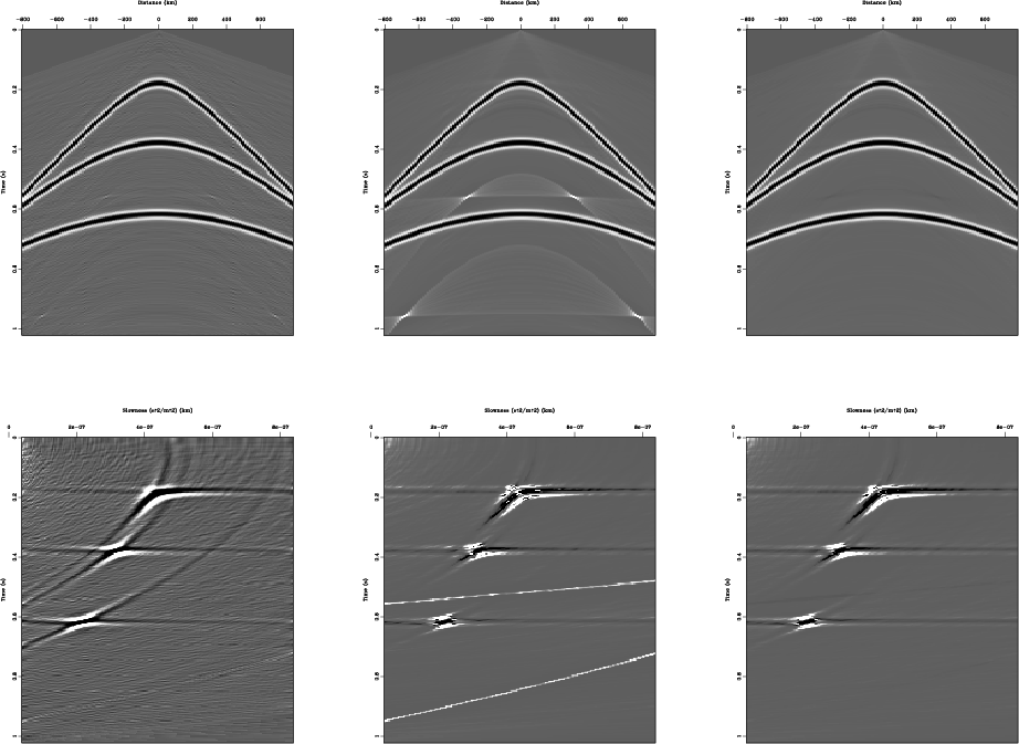
Figures 4d through 4f show the inversion results
obtained using the CGG algorithm with the residual weight only,
the model weight only, and the residual and the model weights together, respectively.
Figures 4a through 4c show the remodeled data
from the corresponding inversion results.
From the results of the residual weight (Figures 4a and 4d),
we can also see the robustness of the residual weight for the busty spike noises,
and also the success in the removal of the Gaussian noise.
Here the residual weight used was the same residual weight as the one used
in the ![]() -norm residual minimizing IRLS method.
Thus we can say that guiding the gradient using the
-norm residual minimizing IRLS method.
Thus we can say that guiding the gradient using the ![]() -norm-like residual weight
in the CGG method seems to behave as the
-norm-like residual weight
in the CGG method seems to behave as the ![]() -norm residual minimizing IRLS method does.
From the results of model weight (Figures 4b and 4e),
we can also see the improvement in the parsimony of the model estimation
compared to the result of LS inversion (Figure 2b)
and the similar behavior in reducing noises as the
-norm residual minimizing IRLS method does.
From the results of model weight (Figures 4b and 4e),
we can also see the improvement in the parsimony of the model estimation
compared to the result of LS inversion (Figure 2b)
and the similar behavior in reducing noises as the ![]() -norm model minimizing IRLS method does.
For the model weight, I used
-norm model minimizing IRLS method does.
For the model weight, I used
![]() , where the exponent 1.5 was decided empirically.
If we want the model weight as the one used in the
, where the exponent 1.5 was decided empirically.
If we want the model weight as the one used in the ![]() -norm model weight in the IRLS method,
the model weight
-norm model weight in the IRLS method,
the model weight
![]() would be
would be ![]() , but the result of it
was not as successful as the IRLS method.
So the appropriate value for the exponent was decided to be
, but the result of it
was not as successful as the IRLS method.
So the appropriate value for the exponent was decided to be ![]() after experiments with several exponent values from 0.5 to 3.
From the results of the residual and model weights together
(Figures 4c and 4f),
we can see that the CGG method also achieves both goals, the robustness to the busty noises
and the parsimony of the model representation, quite well,
and the results of the CGG method are comparable to the results of the IRLS method
(Figures 3c and 3f).
after experiments with several exponent values from 0.5 to 3.
From the results of the residual and model weights together
(Figures 4c and 4f),
we can see that the CGG method also achieves both goals, the robustness to the busty noises
and the parsimony of the model representation, quite well,
and the results of the CGG method are comparable to the results of the IRLS method
(Figures 3c and 3f).
Figure 5 shows the differences of the results of the IRLS method and of the CGG method from the original synthetic data, respectively. We can see that both differences contain nothing but the noise part of data. This demonstrates that both the IRLS method and the CGG methods are very successful in removing various types of noises. Therefore, we can say that the CGG inversion method can be used to achieve the same goal to make an inversion robust and to produce parsimonious model estimation as the IRLS method does. In addition, the CGG method requires less computation than the IRLS method by solving a linear inversion problem (which requires one iteration loop) instead of solving a nonlinear inversion problem (which requires two nested iteration loops).
|
|---|
|
syn-IRLS
Figure 3. The remodeled data and the velocity-stack inversion results obtained by IRLS method with three different norm criteria : (a) and (d) are for the |
|
|
|
|---|
|
syn-CGG
Figure 4. The remodeled data and the velocity-stack inversion results obtained by CGG method with three different guiding weights : (a) and (d) are for the residual weight only, (b) and (e) are for the model weight only, and (c) and (f) are for the residual/model weights together. |
|
|
|
|---|
|
syn-diff
Figure 5. (a) The difference of the remodeled data obtained by IRLS method from the original synthetic data: the original noisy synthetic data (Figure 1) was subtracted from the remodeled data with IRLS method (Figure 3c), (b) The difference of the remodeled data obtained by CGG method from the original synthetic data: the original noisy synthetic data (Figure 1) was subtracted from the remodeled data with CGG method (Figure 4c). |
|
|
|
|
|
|
Conjugate guided gradient (CGG) method for robust inversion and its application to velocity-stack inversion |