|
|
|
|
Nonstationary pattern-based signal-noise separation using adaptive prediction-error filter |
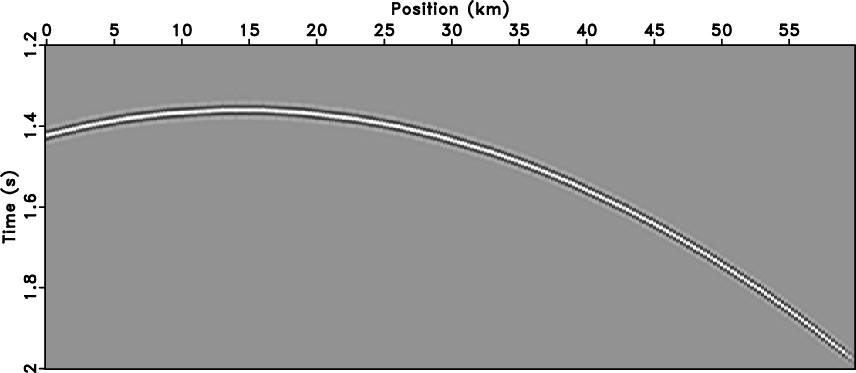
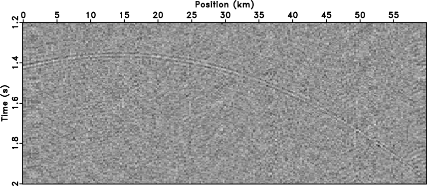
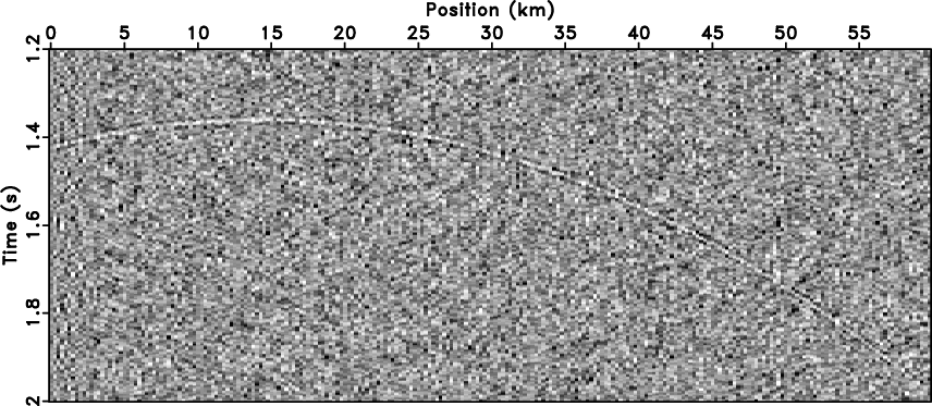
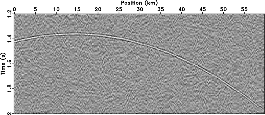
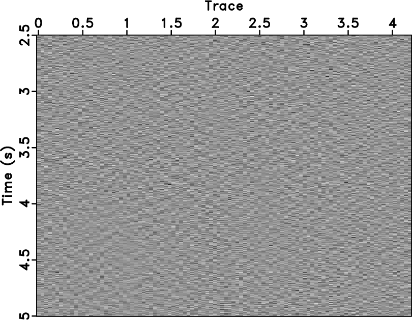
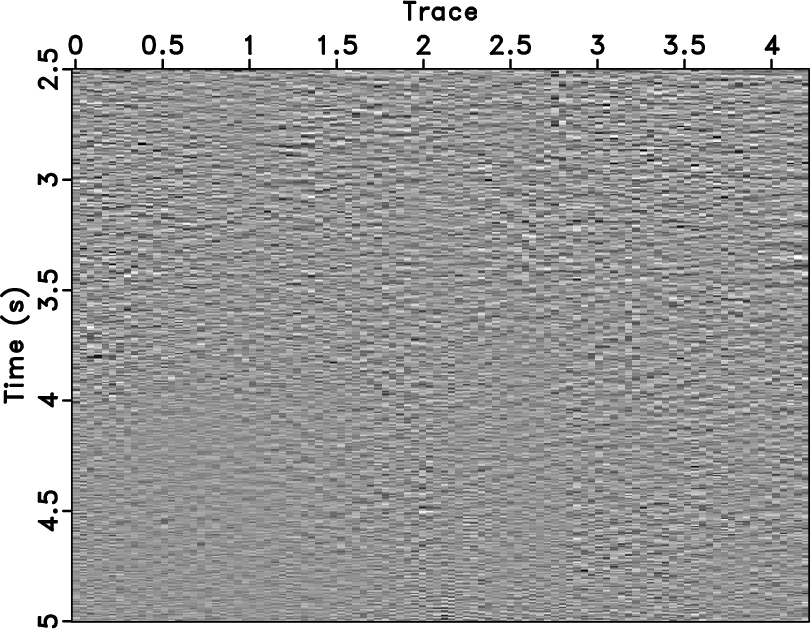
We started with a synthetic model (figure 1a) containing a curve
event with varying slope. Figure 1b is the model data with the white
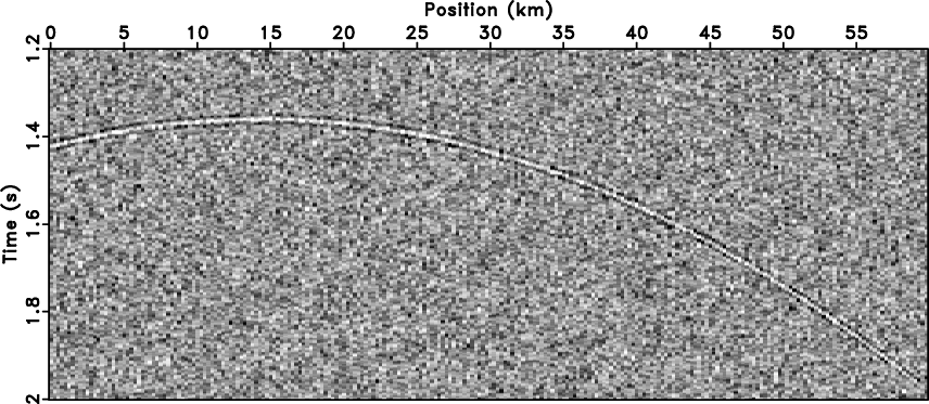
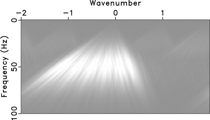
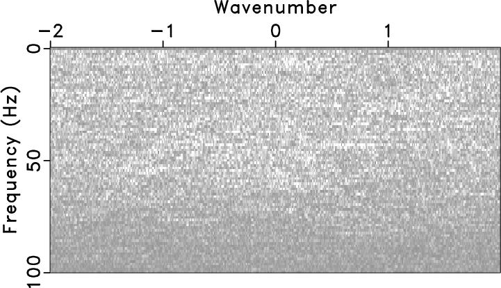
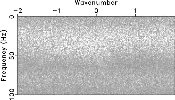
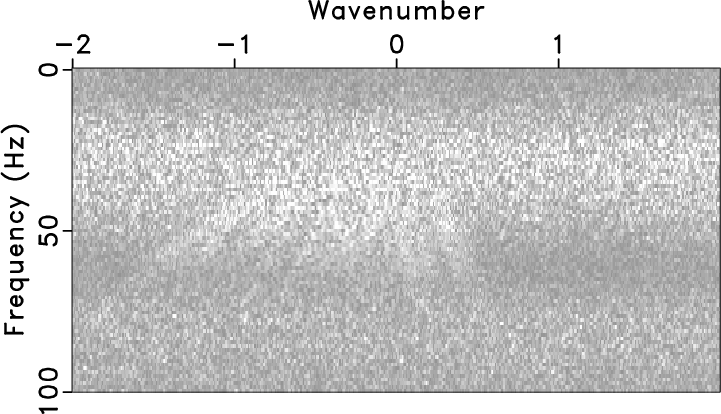
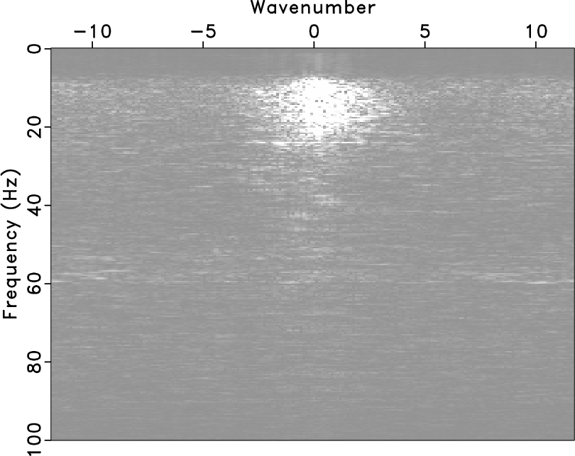
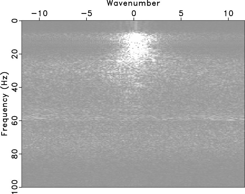
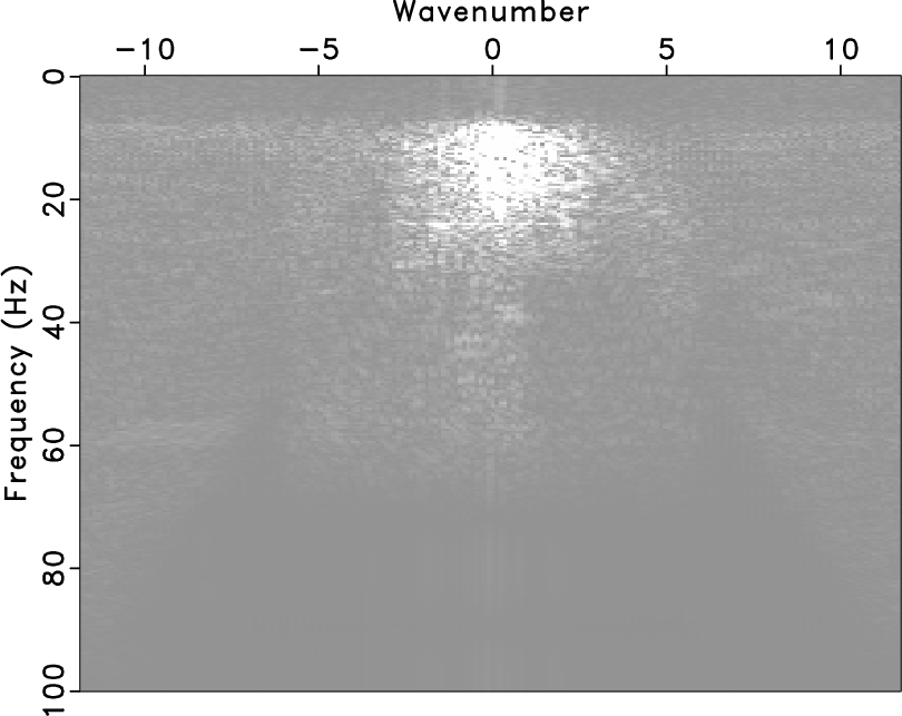
Gaussian noise added. The F-K spectra (figure 2) show
that the strong random noise severely affects the curve model. For comparison,
we first used FXDECON, a standard industry method, to separate the
signal from the noisy data. We designed the FXDECON with four-sample
(space) filter size and ten-sample (space) sliding window. Although
the FXDECON method results in a highest SNR (Table 1), it still fails
to deal with strong random noise. The strong random noise has been
suppressed in the estimated signal section (figure 3a), but a large
part of signal is also destroyed and leaves the estimated noise
section (figure 3b). Due to the strong energy of the random noise,
the high SNR is caused by the suppression of both noise and signal.
To demonstrate the effectiveness of the proposed nonstationary APEF,
we separated the random noise using the pattern-based method
(equation 7) with the stationary PEF in the t-x domain.
The filter size of data pattern (PEF) D is selected with 11 (time)
![]() 4 (space), noise pattern (PEF) N is 5 (time)
4 (space), noise pattern (PEF) N is 5 (time) ![]() 1
(space) coefficients. Figure 3c shows that the stationary approach
fails in separating the random noise in the estimated signal section
as the stationary PEF is hard to characterize the nonstationary data
pattern. Meanwhile, some energy appears from the signal in the estimated
noise section (figure 3d). Figure 3e shows the
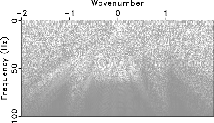
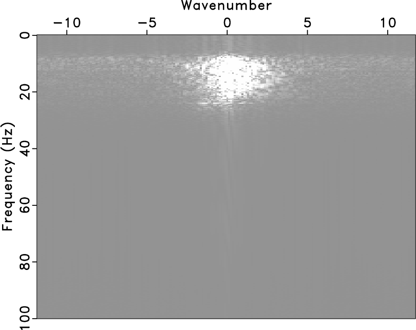
denoised result of the curvelet transform with percentage threshold;
this method effectively suppresses the random noise in the range from
about 30 to 100 Hz (figure 4c), but it generates
striped noise interference that affects the quality of the synthetic model.
For the proposed method, we configured the APEF with the same filter
size as that of the stationary PEF. The smoothing radii in the time
and space directions for data pattern (APEF)
1
(space) coefficients. Figure 3c shows that the stationary approach
fails in separating the random noise in the estimated signal section
as the stationary PEF is hard to characterize the nonstationary data
pattern. Meanwhile, some energy appears from the signal in the estimated
noise section (figure 3d). Figure 3e shows the
denoised result of the curvelet transform with percentage threshold;
this method effectively suppresses the random noise in the range from
about 30 to 100 Hz (figure 4c), but it generates
striped noise interference that affects the quality of the synthetic model.
For the proposed method, we configured the APEF with the same filter
size as that of the stationary PEF. The smoothing radii in the time
and space directions for data pattern (APEF)
![]() is selected
to be 30 and 15 samples, respectively. And the noise pattern (APEF)
is selected
to be 30 and 15 samples, respectively. And the noise pattern (APEF)
![]() has a 300-sample (time)
has a 300-sample (time) ![]() 1-sample (space) smoothing
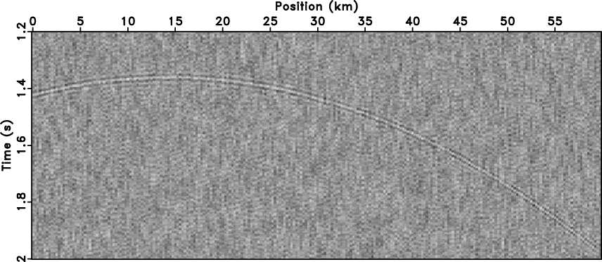
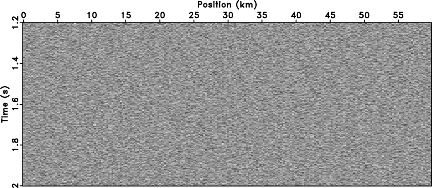
radius. Figure 3g contains a part of the low-level noise,
while the curve event has been recovered. The proposed method shows
better signal protection ability, and obtains the denoised result
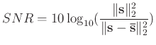
at a high SNR level (Table 1). Here the SNR is
calculated by equation 13:
1-sample (space) smoothing
radius. Figure 3g contains a part of the low-level noise,
while the curve event has been recovered. The proposed method shows
better signal protection ability, and obtains the denoised result
at a high SNR level (Table 1). Here the SNR is
calculated by equation 13:
| Synthetic model | FXDECON | Stationary PEF | Curvelet transform |
|
||||||||||
| SNR | -9.432 | -3.957 | -5.176 | -5.414 | -5.029 |
|
|---|
|
cm-data,cm-noiz
Figure 1. (a) Clean data with curve event and (b) data with random noise. |
|
|

|
|---|
|
cm-fkdata,cm-fknoiz
Figure 2. (a) F-K spectra of clean data and (b) noisy data. |
|
|


|
|---|
|
cm-fx,cm-fxnoiz,cm-pef,cm-pefnoiz,cm-ct,cm-ctnoiz,cm-apef,cm-apefnoiz
Figure 3. (a) Estimated signal and (b) random noise by the FXDECON. (c) Estimated signal and (d) random noise by the pattern-based method with the stationary PEF. (e) Estimated signal and (f) random noise by the curvelet transform. (g) Estimated signal and (h) random noise by the proposed method. |
|
|
|
|---|
|
cm-fkfx,cm-fkpef,cm-fkct,cm-fkapef
Figure 4. (a)F-K spectrum of the denoised result using the FXDECON. (b) F-K spectrum of the denoised result using the pattern-based method with the stationary PEF. (c) F-K spectrum of the denoised result using the curvelet transform. (d) F-K spectrum of the denoised result using the proposed method. |
|
|
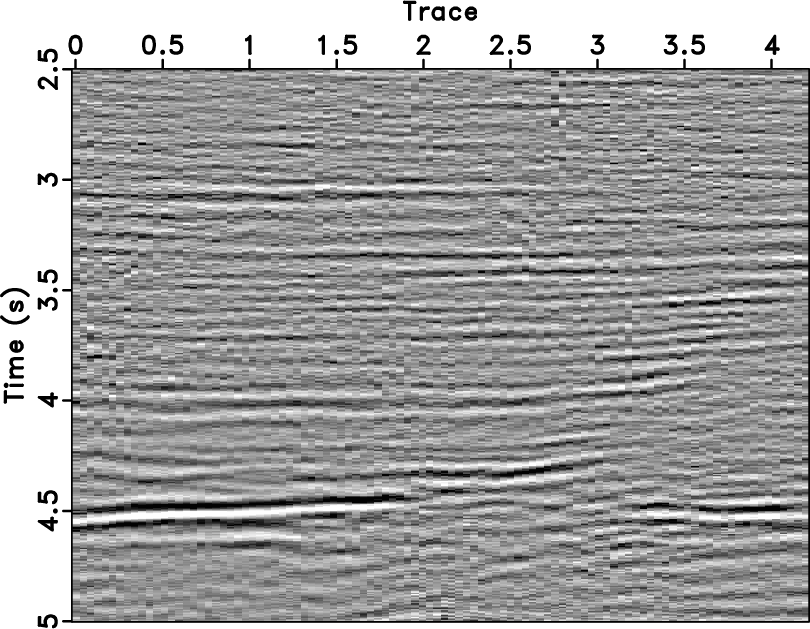
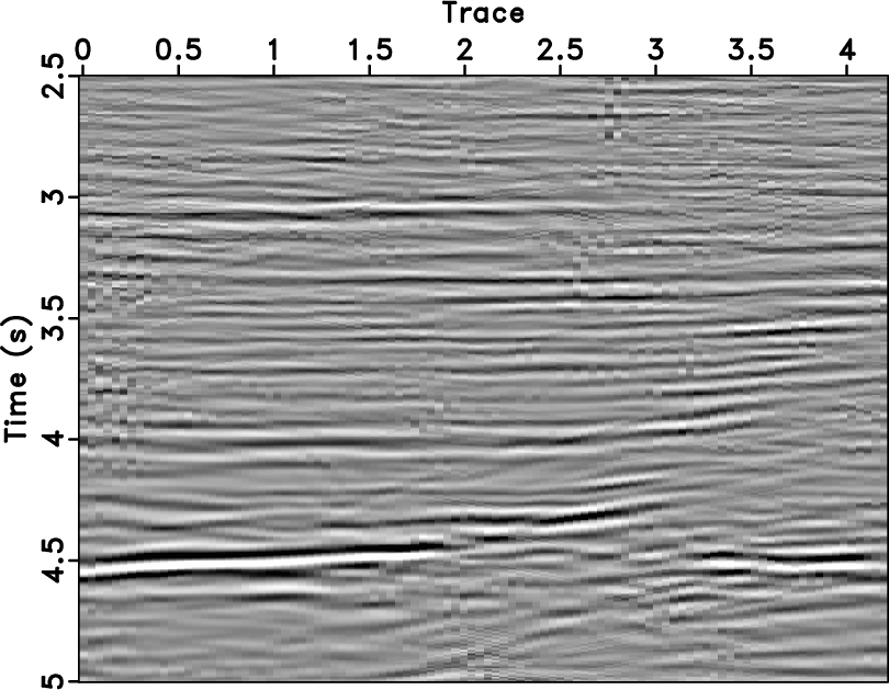
Figure 5 shows a poststack section, where the random
noise influences the continuity of the reflection events. The data includes dipping
beds and a fault. The main challenge in this example is that the random
noise displays the nonstationary energy distribution.
Figure 6 shows the separation results by using FXDECON,
the filter size has eight sample (space) coefficients for each data sample and
a 30-sample (space) sliding window for handling the variation of the
signals. The FXDECON method fails in separating the nonstationary
signal and random noise; weak energy random noise is still present in
the signal section (figure 6a) and part of the
signal leaks into the noise section (figure 6b).
By using the pattern-based method with the stationary PEF, we got
the denoised result in figure 7.
The data pattern (PEF)
![]() is selected with 11 (time)
is selected with 11 (time) ![]() 4 sample (space) coefficients, noise pattern (PEF)
4 sample (space) coefficients, noise pattern (PEF)
![]() has 9
(time)
has 9
(time) ![]() 1 sample (space) coefficients.
In figure 7, the denoised result contains some high
frequency noise, and part of the signal is removed. As shown in figure 10b,
the energy of effective signal at about 18 Hz is partially filtered out.
In the denoised result of curvelet transform with percentage threshold
(figure 8), the random noise causes a stronger smearing of
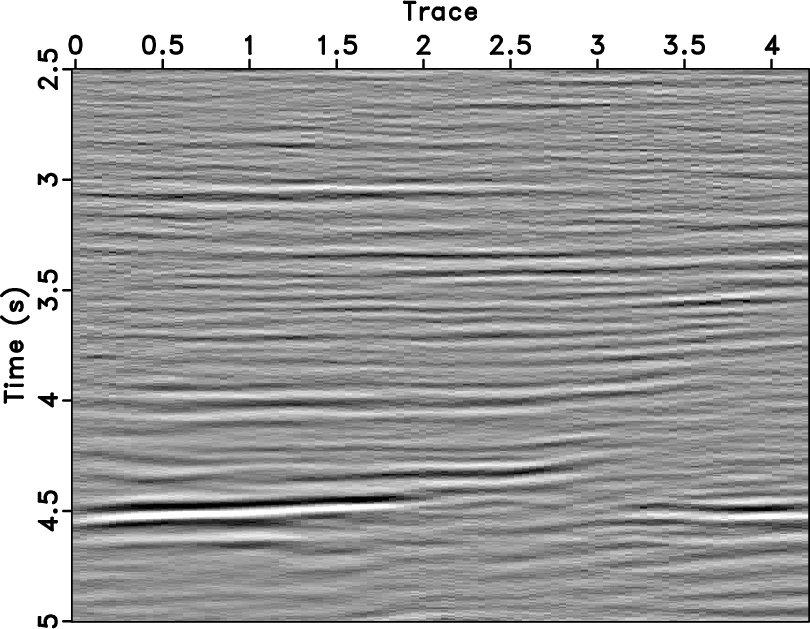
the events. Then we deal with the post- stack section by using the proposed method.
The data APEF
1 sample (space) coefficients.
In figure 7, the denoised result contains some high
frequency noise, and part of the signal is removed. As shown in figure 10b,
the energy of effective signal at about 18 Hz is partially filtered out.
In the denoised result of curvelet transform with percentage threshold
(figure 8), the random noise causes a stronger smearing of
the events. Then we deal with the post- stack section by using the proposed method.
The data APEF
![]() has 9 (time)
has 9 (time) ![]() 4 sample (space)
coefficients for each sample and the smoothing radius is selected to
be 60 (time) and 20 samples (space). The noise APEF
4 sample (space)
coefficients for each sample and the smoothing radius is selected to
be 60 (time) and 20 samples (space). The noise APEF
![]() is
designed as a 9 (time)
is
designed as a 9 (time) ![]() 1 sample (space) coefficients with a
60 (time)
1 sample (space) coefficients with a
60 (time) ![]() 1 sample (space) smoothing radius. The estimated
signal section displays that the continuity of the reflection layers
with better smoothness is enhanced, and the fault is well preserved
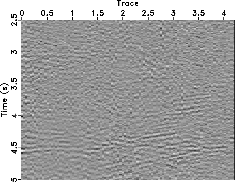
(figure 9a). The energy of the events and fault hardly
leak into the noise section (figure 9b).
The F-K spectrum in figure 10d is cleaner and the effective signal
energy is concentrated. It indicates that the proposed method has a
better capability for noise suppression and signal protection than
other methods.
1 sample (space) smoothing radius. The estimated
signal section displays that the continuity of the reflection layers
with better smoothness is enhanced, and the fault is well preserved
(figure 9a). The energy of the events and fault hardly
leak into the noise section (figure 9b).
The F-K spectrum in figure 10d is cleaner and the effective signal
energy is concentrated. It indicates that the proposed method has a
better capability for noise suppression and signal protection than
other methods.

|
|---|
|
nmo-data,nmo-fkdata
Figure 5. (a) Poststack section with random noise and (b) the corresponding F-K spectrum. |
|
|


|
|---|
|
nmo-fx,nmo-fxnoiz
Figure 6. Random noise separation results of the poststack section using the FXDECON. (a) Section of estimated signal and (b) section of separated random noise. |
|
|
|
|---|
|
nmo-hpef,nmo-hpefnoiz
Figure 7. Random noise separation results of the poststack section using the pattern-based method with the stationary PEF. (a) Section of estimated signal and (b) section of separated random noise. |
|
|
|
|---|
|
nmo-ct,nmo-ctnoiz
Figure 8. Random noise separation results of the poststack section using the curvelet transform. (a) Section of estimated signal and (b) section of separated random noise. |
|
|

|
|---|
|
nmo-apef,nmo-apefnoiz
Figure 9. Random noise separation results of the poststack section using the proposed method. (a) Section of estimated signal and (b) section of separated random noise. |
|
|
|
|---|
|
nmo-fkfx,nmo-fkhpef,nmo-fkct,nmo-fkapef
Figure 10. (a)F-K spectrum of the denoised result using the FXDECON. (b) F-K spectrum of the denoised result using the pattern-based method with the stationary PEF. (c) F-K spectrum of the denoised result using the curvelet transform. (d) F-K spectrum of the denoised result using the proposed method. |
|
|
|
|
|
|
Nonstationary pattern-based signal-noise separation using adaptive prediction-error filter |