|
|
|
|
Seismic data interpolation using streaming prediction filter in the frequency domain |
We first discussed the value selection of the weights
![]() ,
,
![]() , and
, and
![]() . Currently, we considered them as
empirical parameters, but there are still some ways to determine their
value range. 1) In Eq. (10)
and (16),
. Currently, we considered them as
empirical parameters, but there are still some ways to determine their
value range. 1) In Eq. (10)
and (16), ![]() and
and
![]() (or
(or
![]() ) are the
denominator of the filter update term. It is expected that
) are the
denominator of the filter update term. It is expected that
![]() can influence the filter update, so
can influence the filter update, so ![]() and
and
![]() (or
(or
![]() ) should have a
similar order of magnitude, where
) should have a
similar order of magnitude, where
![]() (or
(or
![]() ). 2) In terms of the prediction
filtering theory in the frequency domain, the filter predicts the data
sample along the spatial direction, not along the frequency
direction.
). 2) In terms of the prediction
filtering theory in the frequency domain, the filter predicts the data
sample along the spatial direction, not along the frequency
direction.
![]() and
and
![]() in the spatial direction
should be similar, and their values can be scaled according to the
size of dataset.
in the spatial direction
should be similar, and their values can be scaled according to the
size of dataset.
![]() mainly stabilizes the filter in the
frequency direction, and it generally smaller than
mainly stabilizes the filter in the
frequency direction, and it generally smaller than
![]() and
and
![]() . 3) The regularization terms' weight affect the data
interpolation result to a certain extent. The values of
. 3) The regularization terms' weight affect the data
interpolation result to a certain extent. The values of
![]() ,
,
![]() , and
, and
![]() can be set according to the previous
method, and then they can be adjusted according to the interpolation
effect.
can be set according to the previous
method, and then they can be adjusted according to the interpolation
effect.
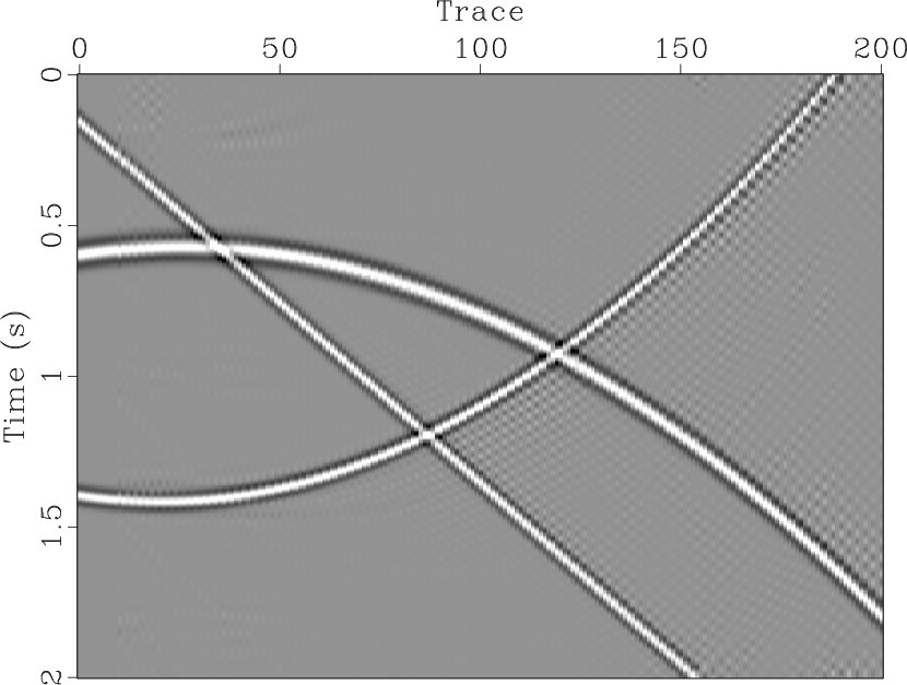
For the case of regular decimation, we tested the synthetic 2D and 3D
model in Fig. 19 and 20. In
the 2D case, we used ten seismic traces to initialize the ![]() -
-![]() SPF,
in which the filter could reconstruct the missing data. As shown in
Fig. 19b, the artifacts affect the data interpolation
quality for traces with large slope differences between the seismic
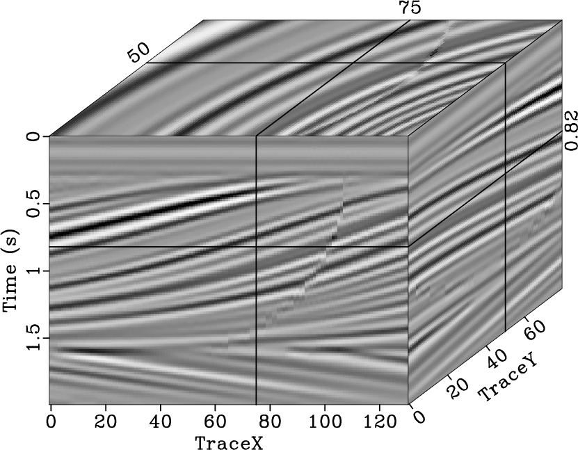
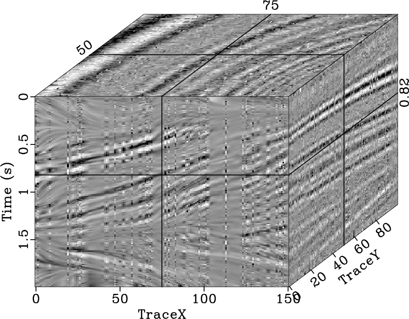
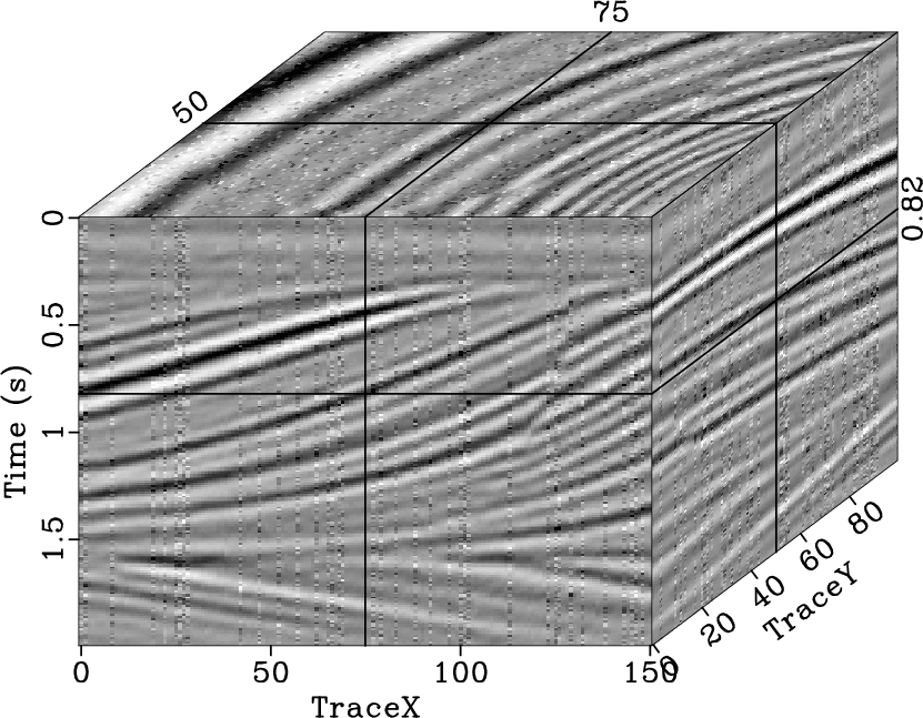
events. For the 3D data (Fig. 20), the
SPF,
in which the filter could reconstruct the missing data. As shown in
Fig. 19b, the artifacts affect the data interpolation
quality for traces with large slope differences between the seismic
events. For the 3D data (Fig. 20), the
![]() -
-![]() -
-![]() SPF can directly recover the missing traces. Although the
regular decimation of the 3D model has strong spatial aliasing, we
still obtained a reasonable interpolation result.
SPF can directly recover the missing traces. Although the
regular decimation of the 3D model has strong spatial aliasing, we
still obtained a reasonable interpolation result.

|
|---|
|
alias,intp
Figure 19. Regular decimation of synthetic 2D model (a), and interpolated result using the 2D |
|
|

|
|---|
|
aliasqd,intpqd
Figure 20. Regular decimation of synthetic 3D model (a), and interpolated result using the 3D |
|
|
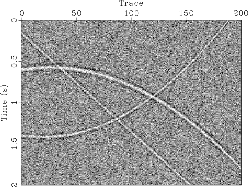
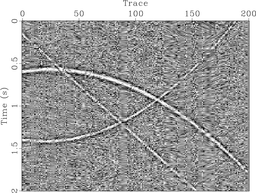
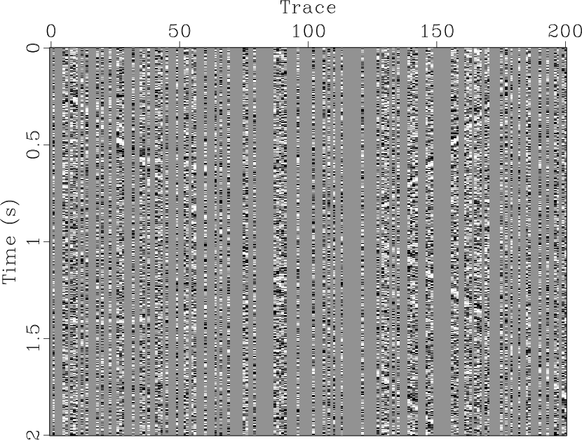
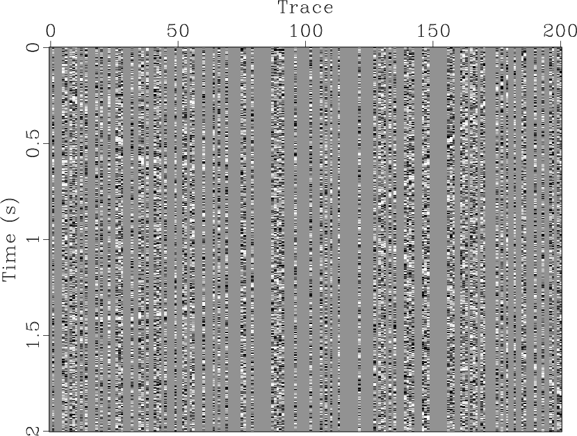
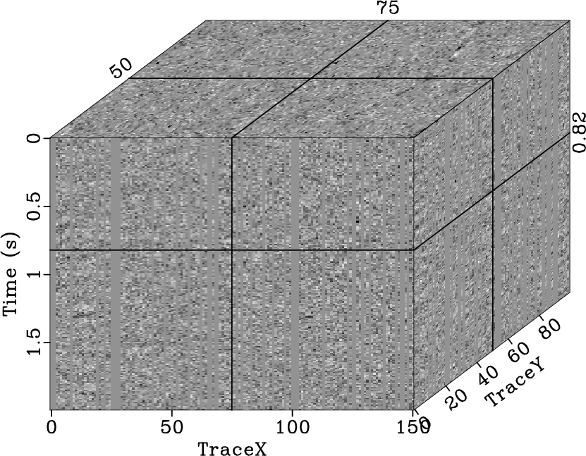
We also tested the effectiveness of the proposed method in the case of
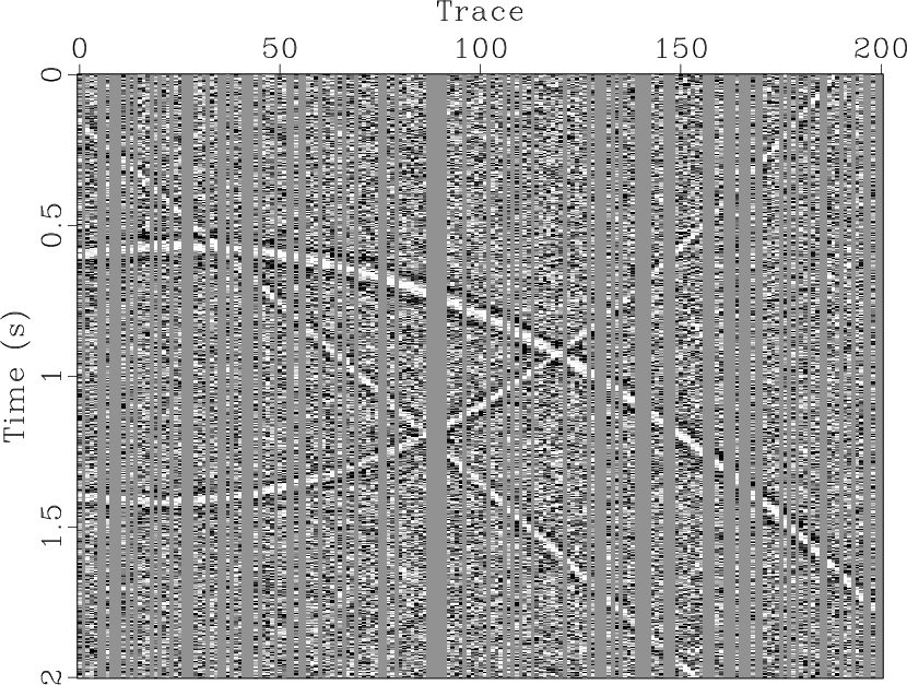
low SNR. We added stronger noise to both the 2D and 3D synthetic
model (Fig. 21a and 23a), which both
had randomly decimated seismic traces. The strong random noise
influenced the local slope calculation, which further affected the
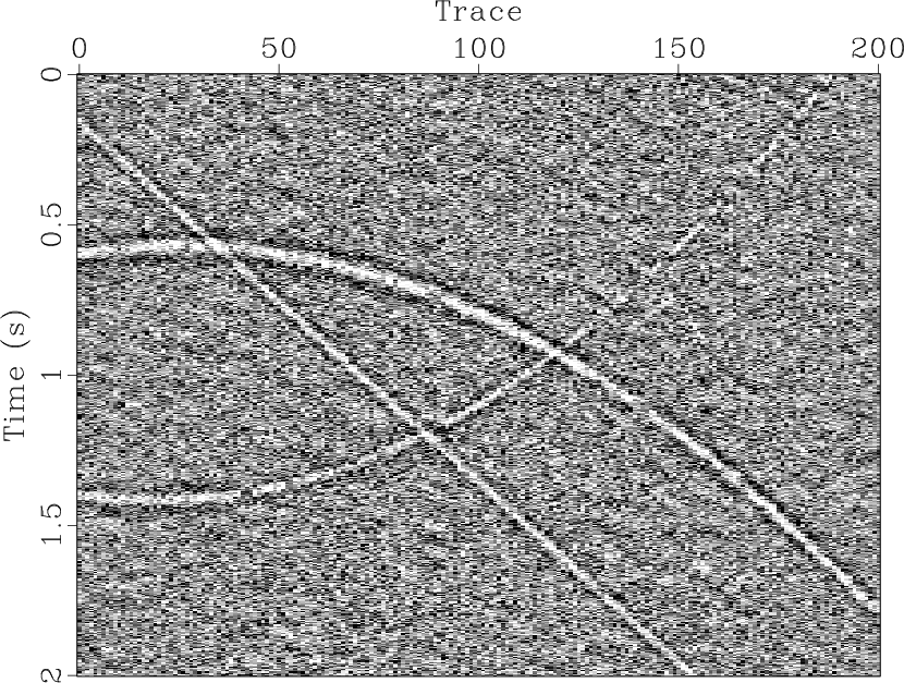
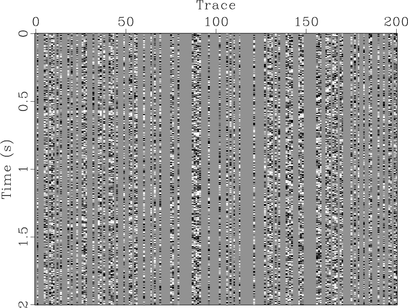
seislet transform. By using the 2D seislet POCS, the interpolation
result of the 2D model (Fig. 22a
and 22b) shows some smearing, and the 3D model
cannot be reconstructed (Fig. 24a
and 24b). For the 2D Fourier POCS method,
there are some parts of the upward curve that are not recovered in the
2D model (Fig. 22c
and 22d). Additionally, the 3D Fourier POCS method
produces a reasonable reconstruction result
(Fig. 24c), although leakage signal of the seismic
events presents in the interpolation error profile
(Fig. 24d). Because the PF can be used to
attenuate random noise, and it may reduce the impact of random noise
to some extent, our proposed methods (the ![]() -
-![]() SPF and the
SPF and the
![]() -
-![]() -
-![]() SPF) yield better reconstruction results
(Fig. 22e, 22f,
24e, and 24f) under low SNR than
other methods.
SPF) yield better reconstruction results
(Fig. 22e, 22f,
24e, and 24f) under low SNR than
other methods.
|
|---|
|
noisemod,noisegap
Figure 21. Synthetic model with random noise (a), model with 40% of the data traces randomly removed (b). |
|
|

|
|---|
|
noisestpocs,noiseerrstpocs,noisepocs,noiseerrpocs,noisefxspf,noiseerrfxspf
Figure 22. Reconstructed result (a) and interpolation error (b) using the 2D seislet POCS, Reconstructed result (c) and interpolation error (d) using the 2D Fourier POCS, reconstructed result (e) and interpolation error (f) using the 2D |
|
|


|
|---|
|
noiseqdome,noisegapqd
Figure 23. Synthetic 3D model with random noise (a), model with |
|
|


|
|---|
|
noisestpocsqd,noiseerrstpocsqd,noisepocsqd,noiseerrpocsqd,noisespfqd,noiseerrspfqd
Figure 24. Reconstructed result (a) and interpolation error (b) using the 2D seislet POCS, reconstructed result (c) and interpolation error (d) using the 3D Fourier POCS, reconstructed result (e) and interpolation error (f) using the 3D |
|
|
|
|
|
|
Seismic data interpolation using streaming prediction filter in the frequency domain |