|
|
|
|
Noniterative f-x-y streaming prediction filtering for random noise attenuation on seismic data |
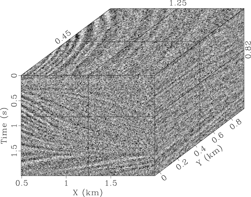
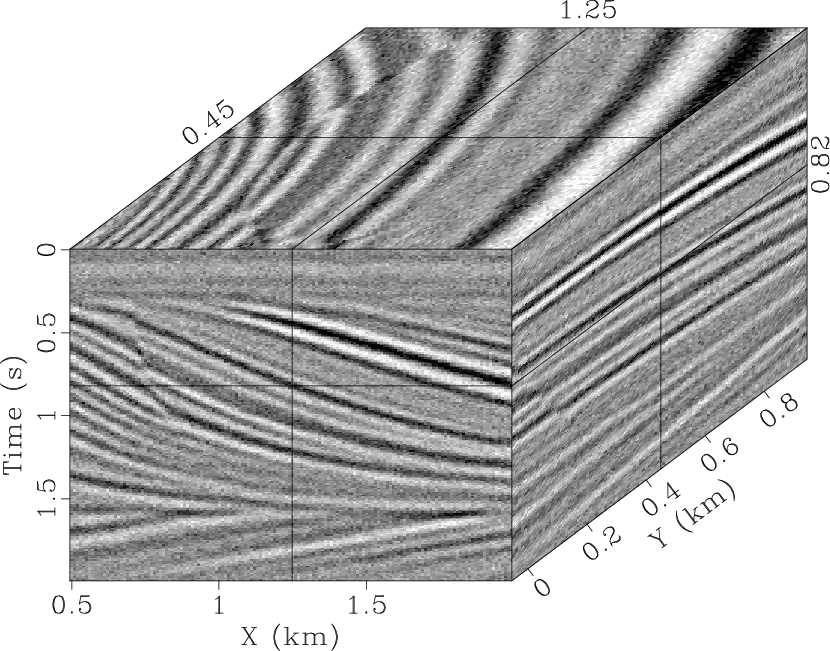
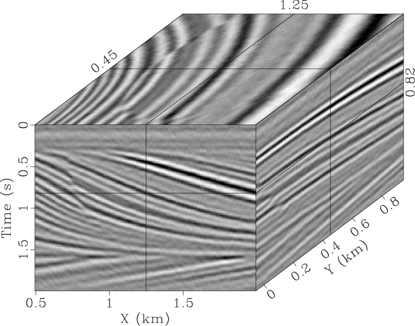
We start with the 3D qdome model Claerbout and Fomel (2008) containing curve
events and faults (Fig. 3a) to evaluate the proposed
method by handling the nonstationarity problem. The model size is 200
(time samples) ![]() 150 (X traces)
150 (X traces) ![]() 100 (Y traces).
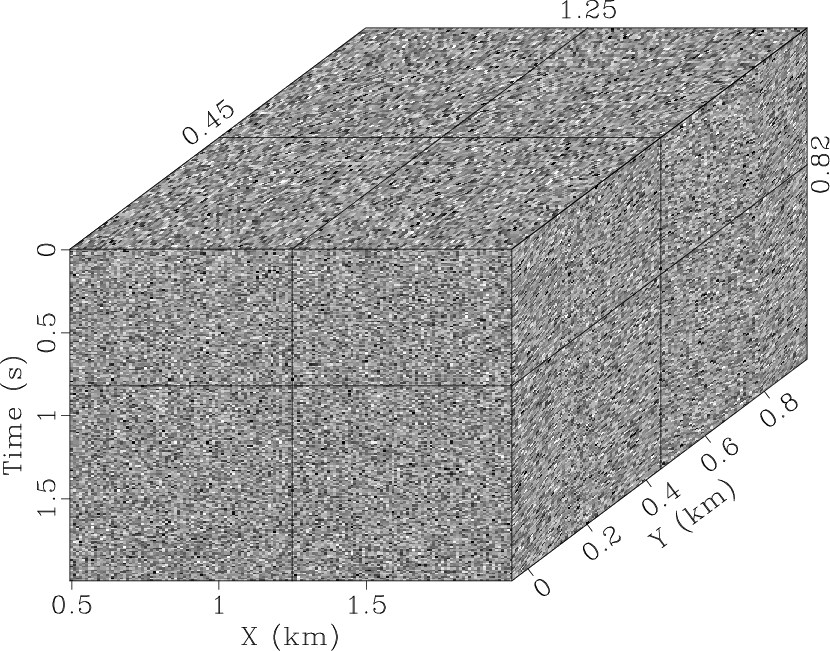
Fig. 3b displays the data with Gaussian noise added.
We compared the 3D
100 (Y traces).
Fig. 3b displays the data with Gaussian noise added.
We compared the 3D ![]() -
-![]() -
-![]() SPF with the 2D
SPF with the 2D ![]() -
-![]() SPF and the 3D
SPF and the 3D
![]() -
-![]() -
-![]() RNA Liu and Chen (2013) to test their ability for random noise
attenuation. The filter length of the
RNA Liu and Chen (2013) to test their ability for random noise
attenuation. The filter length of the ![]() -
-![]() SPF is 5-sample
(
SPF is 5-sample
(![]() ). We also selected the scale parameters with 0.008
(
). We also selected the scale parameters with 0.008
(
![]() ) and 0.06 (
) and 0.06 (
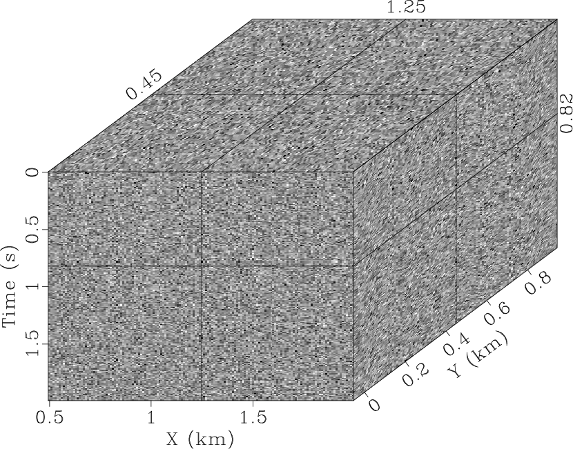
![]() ). Fig. 4a shows
the denoised result obtained by using the
). Fig. 4a shows
the denoised result obtained by using the ![]() -
-![]() SPF that eliminates
most of the random noise. However, there is still an obvious signal in
the noise section (Fig. 4b) because the 2D
SPF that eliminates
most of the random noise. However, there is still an obvious signal in
the noise section (Fig. 4b) because the 2D ![]() -
-![]() SPF has a low accuracy owing to the local similarity of filter
coefficients only along the
SPF has a low accuracy owing to the local similarity of filter
coefficients only along the ![]() and
and ![]() directions. A more effective
approach is to apply global smoothness. The denoised result obtained
by using the 3D
directions. A more effective
approach is to apply global smoothness. The denoised result obtained
by using the 3D ![]() -
-![]() -
-![]() RNA is shown in Fig. 4c. The
filter size of the
RNA is shown in Fig. 4c. The
filter size of the ![]() -
-![]() -
-![]() RNA is 5-sample (
RNA is 5-sample (![]() )
) ![]() 5-sample
(
5-sample
(![]() ). The 3D
). The 3D ![]() -
-![]() -
-![]() RNA has a better result than the 2D
RNA has a better result than the 2D ![]() -
-![]() SPF, and it is visually difficult to detect the signal in the
difference between the noisy data (Fig. 3b) and the
denoised result (Fig. 4c). The global smoothness
constraints along two spatial directions can help RNA to improve the
result (Fig. 4d), but it also increases the
computational cost because it iteratively solves the regularized
least-squares problem (Table 1). We designed a 3D
SPF, and it is visually difficult to detect the signal in the
difference between the noisy data (Fig. 3b) and the
denoised result (Fig. 4c). The global smoothness
constraints along two spatial directions can help RNA to improve the
result (Fig. 4d), but it also increases the
computational cost because it iteratively solves the regularized
least-squares problem (Table 1). We designed a 3D
![]() -
-![]() -
-![]() SPF with 5-sample (
SPF with 5-sample (![]() )
) ![]() 5-sample (
5-sample (![]() )
coefficients for each sample and the scale parameters 0.008
(
)
coefficients for each sample and the scale parameters 0.008
(
![]() ), 0.06 (
), 0.06 (
![]() ), and 0.06 (
), and 0.06 (
![]() ). The
proposed method produces a reasonable result (Fig. 4e),
where the geological structure is improved. It is also difficult to
distinguish the signal in the removed noise
(Fig. 4f), which is an indication of successful
signal and noise separation. The signal-to-noise ratio (SNR) and time
consumption were used to analyze the performance of each method
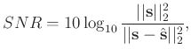
(Table 2). The SNR is defined as:
). The
proposed method produces a reasonable result (Fig. 4e),
where the geological structure is improved. It is also difficult to
distinguish the signal in the removed noise
(Fig. 4f), which is an indication of successful
signal and noise separation. The signal-to-noise ratio (SNR) and time
consumption were used to analyze the performance of each method
(Table 2). The SNR is defined as:


|
|---|
|
qdmod,qdnoise
Figure 3. 3D synthetic model (a) and noisy data (b). |
|
|

|
|---|
|
qdspf2,qderrspf2,qdrna,qderrrna,qdspf3,qderrspf3
Figure 4. Denoised result by the |
|
|
|
|
|
|
Noniterative f-x-y streaming prediction filtering for random noise attenuation on seismic data |