|
|
|
|
Noniterative f-x-y streaming prediction filtering for random noise attenuation on seismic data |
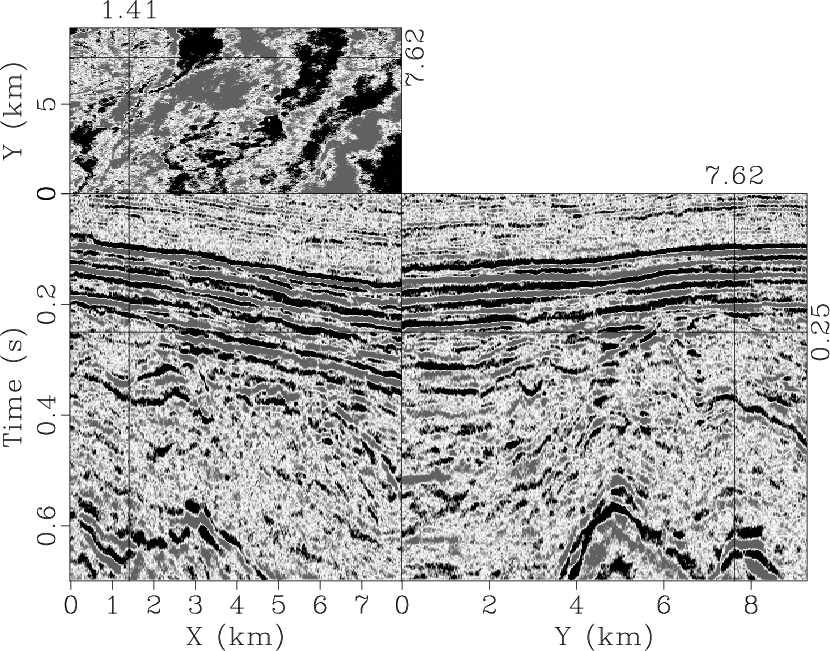
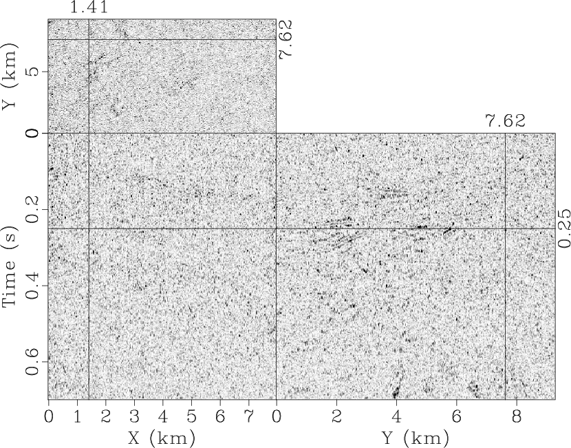
For the field data test, we used a 3D time migration data to evaluate
the effectiveness of the SPF (Fig. 7). The data size
is 700-sample (time) ![]() 266-sample (X)
266-sample (X) ![]() 310-sample
(Y). Strong random noise from the surface conditions contaminates both
the simple layers at the shallow locations and complex structure at
the deeper positions. We applied the 2D
310-sample
(Y). Strong random noise from the surface conditions contaminates both
the simple layers at the shallow locations and complex structure at
the deeper positions. We applied the 2D ![]() -
-![]() SPF with 5-sample
(
SPF with 5-sample
(![]() ) to recover the events and selected 55 (
) to recover the events and selected 55 (
![]() ) and 280
(
) and 280
(
![]() ) as the regularization terms for the improved
) as the regularization terms for the improved ![]() -
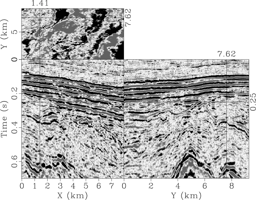
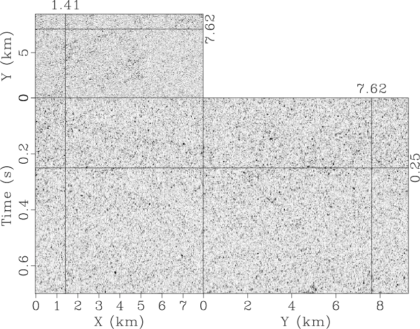
-![]() SPF with frequency constraint. Fig. 8a and
8b show the denoised results and the removed noise
at the same clip value, respectively. Both shallow plane events and
deep dipping events show better lateral continuity, but the 2D SPF
also removes a part of the events because it uses the local smoothness
constraints without the
SPF with frequency constraint. Fig. 8a and
8b show the denoised results and the removed noise
at the same clip value, respectively. Both shallow plane events and
deep dipping events show better lateral continuity, but the 2D SPF
also removes a part of the events because it uses the local smoothness
constraints without the ![]() direction. Meanwhile, information is
removed near
direction. Meanwhile, information is
removed near ![]() and
and ![]() because of the inaccurate initial filter
coefficients. We also compared the 2D SPF with the 2D
because of the inaccurate initial filter
coefficients. We also compared the 2D SPF with the 2D ![]() -
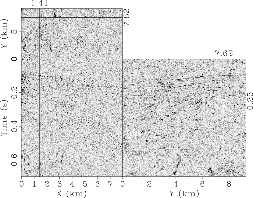
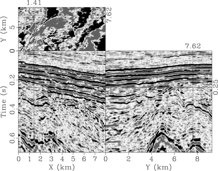
-![]() EMD
prediction filter Chen and Ma (2014) to test it ability for random noise
attenuation. The denoised result of
EMD
prediction filter Chen and Ma (2014) to test it ability for random noise
attenuation. The denoised result of ![]() -
-![]() EMD prediction filter is
shown in Fig. 9a. The 2D
EMD prediction filter is
shown in Fig. 9a. The 2D ![]() -
-![]() EMD prediction
filter preserves signal better than the 2D SPF, but the difference
(Fig. 9b) still shows obvious signal and the
method is difficult to be implemented in 3D case. For comparison, we
used the 3D
EMD prediction
filter preserves signal better than the 2D SPF, but the difference
(Fig. 9b) still shows obvious signal and the
method is difficult to be implemented in 3D case. For comparison, we
used the 3D ![]() -
-![]() -
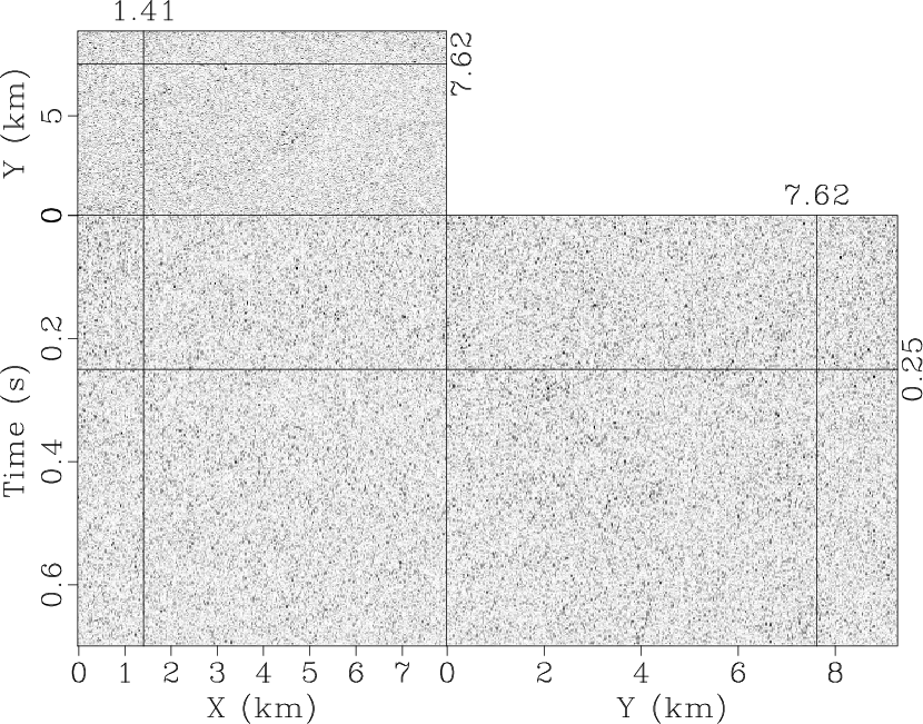
-![]() RNA to attenuate random noise. The
RNA to attenuate random noise. The
![]() -
-![]() -
-![]() RNA with 5-sample (X)
RNA with 5-sample (X) ![]() 5-sample (Y) filter size
outputs a smoother result and the lateral continuity is improved
(Fig. 10a), where the reflection event in both shallow
and deep parts becomes clearer than original field
data. Fig. 10b displays that only parts of dipping
events are slightly lost. The proposed
5-sample (Y) filter size
outputs a smoother result and the lateral continuity is improved
(Fig. 10a), where the reflection event in both shallow
and deep parts becomes clearer than original field
data. Fig. 10b displays that only parts of dipping
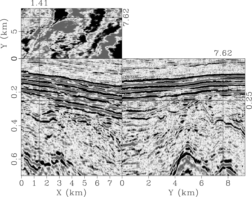
events are slightly lost. The proposed ![]() -
-![]() -
-![]() SPF can produce
more feasible results than the 2D version because the 3D SPF has extra
nonstationarity along the
SPF can produce
more feasible results than the 2D version because the 3D SPF has extra
nonstationarity along the ![]() axis (Fig. 11a), where
the continuity of the events and the geological structure are
enhanced. The scale parameters are selected as 90 (
axis (Fig. 11a), where
the continuity of the events and the geological structure are
enhanced. The scale parameters are selected as 90 (
![]() ), 600
(
), 600
(
![]() ), and 600 (
), and 600 (
![]() ) and the same 5-sample (X)
) and the same 5-sample (X)
![]() 5-sample (Y) filter size as the 3D
5-sample (Y) filter size as the 3D ![]() -
-![]() -
-![]() RNA. The
difference (Fig. 11b) between the noisy data
(Fig. 7) and the denoised result
(Fig. 11a) shows more uniformly-distributed random
noise than the 3D
RNA. The
difference (Fig. 11b) between the noisy data
(Fig. 7) and the denoised result
(Fig. 11a) shows more uniformly-distributed random
noise than the 3D ![]() -
-![]() -
-![]() RNA, which demonstrates that the
proposed filter is able to depict the variations in the nonstationary
signals and provide an accurate estimation of complex wavefields even
in the presence of strongly curved and conflicting events.
Furthermore, the
RNA, which demonstrates that the
proposed filter is able to depict the variations in the nonstationary
signals and provide an accurate estimation of complex wavefields even
in the presence of strongly curved and conflicting events.
Furthermore, the ![]() -
-![]() -
-![]() SPF takes relatively low computational
time (Table 2) that highlights its efficiency,
especially in higher dimensions.
SPF takes relatively low computational
time (Table 2) that highlights its efficiency,
especially in higher dimensions.
|
|---|
|
realdata
Figure 7. Three-dimensional field data. |
|
|
|
|---|
|
realspf2,realerrspf2
Figure 8. The denoised result by using the 2D |
|
|
|
|---|
|
realfxemd,realerrfxemd
Figure 9. The denoised result by using the |
|
|

|
|---|
|
realrna,realerrrna
Figure 10. The denoised result by using the 3D |
|
|
|
|---|
|
realspf3,realerrspf3
Figure 11. The denoised result by using the 3D |
|
|
|
|
|
|
Noniterative f-x-y streaming prediction filtering for random noise attenuation on seismic data |