|
|
|
|
Velocity-independent |
|
|---|
|
dataSynth
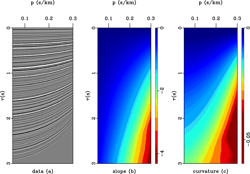
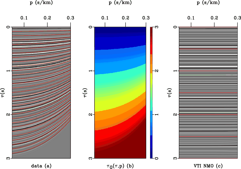
Figure 3. (a) A synthetic |
|
|
We first test our method on a synthetic example, where the exact
velocity model is known. The example is introduced in Figure
3. The synthetic data were generated by applying
inverse ![]() -
-![]() NMO with time-variable effective velocities. Both the
effective NMO
NMO with time-variable effective velocities. Both the
effective NMO ![]() and horizontal
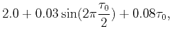
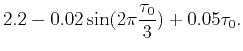
and horizontal ![]() velocity increase
linearly with vertical time and include a sinusoidal change with time,
as described by the following relations
velocity increase
linearly with vertical time and include a sinusoidal change with time,
as described by the following relations
 |
|||
 |
The CMP maximum offset-to-depth ratio is nearly 2.0 for large
value of the horizontal slope ![]() . This should guarantee the necessary
data sensitivity for resolving high-order moveout parameters
(Tsvankin, 2006). Figure 3b shows local event
slopes
. This should guarantee the necessary
data sensitivity for resolving high-order moveout parameters
(Tsvankin, 2006). Figure 3b shows local event
slopes ![]() measured from the data using the plane-wave destruction
(PWD) algorithm (see Appendix A). Plane-wave destruction predicts each
seismic trace from a neighboring one along local slopes. As
explained in appendix A, local slopes are extracted by minimizing the
prediction error in an iterative regularized least-squares
optimization. Shaping regularization controls the smoothness of the
estimated slope field (Fomel, 2007a). If the seismic data are
particularly noisy, a more aggressive regularization can help in
getting a more consistent and stable estimate. For cleaner data, less
smoothing yields a better-resolved and detailed slope field.
measured from the data using the plane-wave destruction
(PWD) algorithm (see Appendix A). Plane-wave destruction predicts each
seismic trace from a neighboring one along local slopes. As
explained in appendix A, local slopes are extracted by minimizing the
prediction error in an iterative regularized least-squares
optimization. Shaping regularization controls the smoothness of the
estimated slope field (Fomel, 2007a). If the seismic data are
particularly noisy, a more aggressive regularization can help in
getting a more consistent and stable estimate. For cleaner data, less
smoothing yields a better-resolved and detailed slope field.
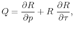
Unlike slopes, we don't directly estimate the curvature field ![]() . We
compute the curvature by simply differentiating the slope
estimate. Since slope
. We
compute the curvature by simply differentiating the slope
estimate. Since slope
![]() depends on both the current ray
parameter
depends on both the current ray
parameter ![]() and the time
and the time
![]() , which is again a function
of
, which is again a function
of ![]() , we compute the derivative of the slope field by a
straightforward application of the chain rule, as follows:
, we compute the derivative of the slope field by a
straightforward application of the chain rule, as follows:
|
|---|
|
dataNMO1
Figure 4. (b) Time mapping of each data sample from |
|
|
Figure 4b represents the zero-slope traveltime ![]() mapped according to the oriented NMO formula in equation
15. These values predict correctly the reflection
trajectories (red lines in Figure 4a) which
then get warped until they are completely flattened (Figure
4c). Moreover, the oriented NMO does not introduce
stretch effects as the traditional NMO processing. This is because
the slope-based NMO applies a locally static shift to each data
sample as opposed to to the dynamic one of the conventional NMO correction.
mapped according to the oriented NMO formula in equation
15. These values predict correctly the reflection
trajectories (red lines in Figure 4a) which
then get warped until they are completely flattened (Figure
4c). Moreover, the oriented NMO does not introduce
stretch effects as the traditional NMO processing. This is because
the slope-based NMO applies a locally static shift to each data
sample as opposed to to the dynamic one of the conventional NMO correction.

|
|---|
|
mapE
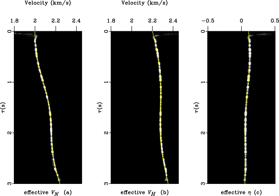
Figure 5. Effective normal moveout velocity (a), horizontal velocity (b) and anellipticity parameter |
|
|
In conventional NMO processing, one scans a number of velocities,
performs the corresponding moveout corrections, and picks the velocity
trend from velocity spectra maxima. In the oriented processing,
according to equations 16-18, anisotropy
parameters become data attributes rather than prerequisites for
imaging. Figure 5 shows the effective ![]() ,
, ![]() and
and ![]() values as data attributes mapped to the correct vertical
time
values as data attributes mapped to the correct vertical
time ![]() position according to equation
15. These parameters have been obtained from the
data through an automatic estimation of the local-slope field. The
computational speed together with the automation are the main
advantages of oriented processing.
position according to equation
15. These parameters have been obtained from the
data through an automatic estimation of the local-slope field. The
computational speed together with the automation are the main
advantages of oriented processing.
Even though this synthetic data is noise-free, the slope and curvature
estimates are not perfect. Nevertheless, Figure 5 shows a
nearly constant trend along ![]() direction of the recovered parameters
that confirms the reliability of our method. Despite the large offset-to-depth ratio, we observe that
direction of the recovered parameters
that confirms the reliability of our method. Despite the large offset-to-depth ratio, we observe that ![]() and
and ![]() are more sensitive to the slope estimate uncertainty, which agrees with
the observation of Tsvankin (2006) that high-order moveout
parameters are in general less constrained than the short-spread
normal moveout velocity
are more sensitive to the slope estimate uncertainty, which agrees with
the observation of Tsvankin (2006) that high-order moveout
parameters are in general less constrained than the short-spread
normal moveout velocity ![]() . The reduced data sensitivity to
. The reduced data sensitivity to
![]() and
and ![]() at short offsets can explain the errors in the
upper-right corner in panels (b) and (c) in Figure 5. A
proper filtering procedure of the parameter maps may allow us to recover accurate parameter trends like
those in Figure 6. The panels in Figure
6 represent semblance-like spectra computed by mapping
each data sample to its parameter value at the zero-slope time
at short offsets can explain the errors in the
upper-right corner in panels (b) and (c) in Figure 5. A
proper filtering procedure of the parameter maps may allow us to recover accurate parameter trends like
those in Figure 6. The panels in Figure
6 represent semblance-like spectra computed by mapping
each data sample to its parameter value at the zero-slope time ![]() . The yellow lines indicate the exact effective-parameter
profiles used to generate the synthetic gather and confirm that our
estimations follow the exact trends. Compared to conventional
semblance spectra, these plots do not show the elongated ``bull's
eye'' patterns which grow with increasing time. The improved
resolution comes from the slope estimation accuracy and relates to the
quality and complexity of the input data.
. The yellow lines indicate the exact effective-parameter
profiles used to generate the synthetic gather and confirm that our
estimations follow the exact trends. Compared to conventional
semblance spectra, these plots do not show the elongated ``bull's
eye'' patterns which grow with increasing time. The improved
resolution comes from the slope estimation accuracy and relates to the
quality and complexity of the input data.
|
|---|
|
eff-Syn
Figure 6. Effective normal moveout velocity (a), horizontal velocity (b) and anellipticity parameter |
|
|
|
|
|
|
Velocity-independent |