|
|
|
|
Inverse B-spline interpolation |
B-splines represent a particular example of a convolutional basis. Because of their compact support and other attractive numerical properties, B-splines are a good basis choice for the forward interpolation problem and related signal processing problems (Unser, 1999).
B-splines of the order 0 and 1 coincide with the nearest neighbor and
linear interpolants (2) and (3) respectively.
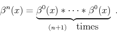
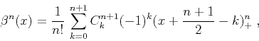
B-splines ![]() of a higher order
of a higher order ![]() can be defined by a
repetitive convolution of the zeroth-order spline
can be defined by a
repetitive convolution of the zeroth-order spline ![]() (the
box function) with itself:
(the
box function) with itself:
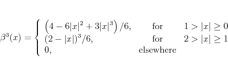
Both the support length and the smoothness of B-splines increase with
the order. In the limit, B-slines converge to the Gaussian function.
Figures 11 and 12 show the third- and
seventh-order splines ![]() and
and ![]() and their
continuous spectra.
and their
continuous spectra.

|
|---|
|
splint3
Figure 11. Third-order B-spline |
|
|

|
|---|
|
splint7
Figure 12. Seventh-order B-spline |
|
|
It is important to realize the difference between B-splines and the
corresponding interpolants ![]() , which are sometimes called
cardinal splines. An explicit computation of the cardinal
splines is impractical, because they have infinitely long support.
Typically, they are constructed implicitly by the two-step
interpolation method, outlined in the previous subsection. The
cardinal splines of orders 3 and 7 and their spectra are shown in
Figures 13 and 14. As B-splines converge
to the Gaussian function, the corresponding interpolants rapidly
converge to the sinc function (4). A good convergence
is achieved with the help of the infinitely long support, which
results from recursive filtering at the first step of the
interpolation procedure.
, which are sometimes called
cardinal splines. An explicit computation of the cardinal
splines is impractical, because they have infinitely long support.
Typically, they are constructed implicitly by the two-step
interpolation method, outlined in the previous subsection. The
cardinal splines of orders 3 and 7 and their spectra are shown in
Figures 13 and 14. As B-splines converge
to the Gaussian function, the corresponding interpolants rapidly
converge to the sinc function (4). A good convergence
is achieved with the help of the infinitely long support, which
results from recursive filtering at the first step of the
interpolation procedure.

|
|---|
|
crdint3
Figure 13. Effective third-order B-spline interpolant (left) and its spectrum (right). |
|
|

|
|---|
|
crdint7
Figure 14. Effective seventh-order B-spline interpolant (left) and its spectrum (right). |
|
|
In practice, the recursive filtering step adds only marginally to the
total interpolation cost. Therefore, an ![]() -th order B-spline
interpolation is comparable in cost with any other method with an
-th order B-spline
interpolation is comparable in cost with any other method with an
![]() -point interpolant. The comparison in accuracy usually turns
out in favor of B-splines. Figures 15
and 16 compare interpolation errors of B-splines and
other similar-cost methods on the example from Figure 4.
-point interpolant. The comparison in accuracy usually turns
out in favor of B-splines. Figures 15
and 16 compare interpolation errors of B-splines and
other similar-cost methods on the example from Figure 4.
|
cubspl4
Figure 15. Interpolation error of the cubic convolution interpolant (dashed line) compared to that of the third-order B-spline (solid line). |

|
|---|---|
|
|
|
kaispl8
Figure 16. Interpolation error of the 8-point windowed sinc interpolant (dashed line) compared to that of the seventh-order B-spline (solid line). |

|
|---|---|
|
|
Similarly to Figures 8 and 9, we can also compare the discrete responses of B-spline interpolation with those of other methods. The right plots in Figures 17 and 18 show that the discrete spectra of the effective B-spline interpolants are genuinely flat at low frequencies and wider than those of the competitive methods. Although the B-spline responses are infinitely long because of the recursive filtering step, they exhibit a fast amplitude decay.
|
speccubspl4
Figure 17. Discrete interpolation responses of cubic convolution and third-order B-spline interpolants (left) and their discrete spectra (right) for |

|
|---|---|
|
|
|
speckaispl8
Figure 18. Discrete interpolation responses of 8-point windowed sinc and seventh-order B-spline interpolants (left) and their discrete spectra (right) for |

|
|---|---|
|
|
|
|
|
|
Inverse B-spline interpolation |