A variational formulation of the fast marching eikonal solver

Mesh Refinement

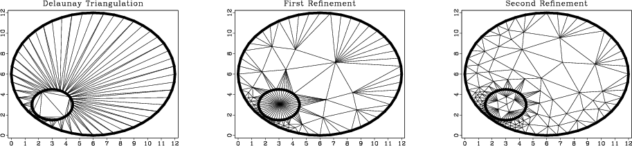
One the main properties of Delaunay triangulation is that, for a given set of nodes, it provides the maximum smallest angle among all possible triangulations. It is this property that supports the wide usage of Delaunay algorithms in the mesh generation problems. However, it doesn't guarantee that the smallest angle will always be small. In fact, for some point distributions, it is impossible to avoid skinny small-angle triangles. The remedy is to add additional nodes to the triangulation so that the quality of the triangles is globally improved. This problem has become known as mesh refinement (Ruppert, 1995).

hole
Figure A-8. An illustration of Rivara's refinement algorithm. The left plot shows an input to the algorithm: a valid Delaunay triangulation with ``skinny'' triangles. Two other plots show successive applications of the refinement algorithm.

One of the recently proposed mesh refinement algorithms is Rivara's backward longest-side refinement technique (Rivara, 1996). The main idea of the algorithm is to trace the LSPP (longest-side propagation path) for each refined triangle. The LSPP is an ordered list of triangles, connected by a common edge, such that the longest triangle edge is strictly increasing. After tracing the LSPP, we bisect the longest edge and insert its midpoint into the triangulation. Rivara's algorithm is remarkably efficient and easy to implement. In comparison with alternative methods, it has the additional advantage of being applicable in three dimensions.

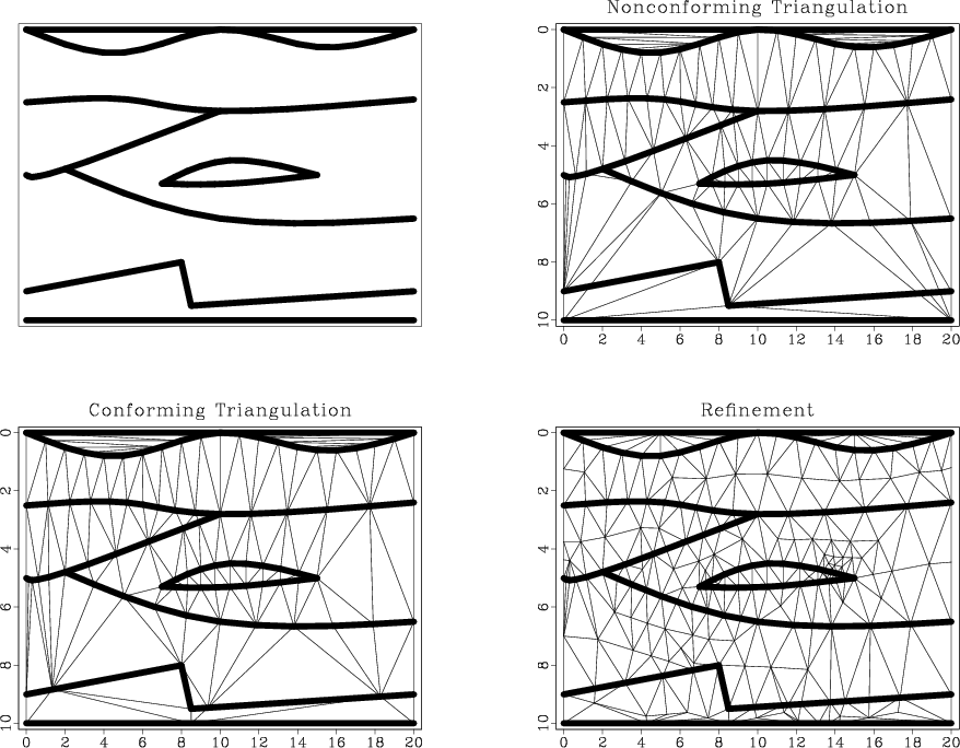
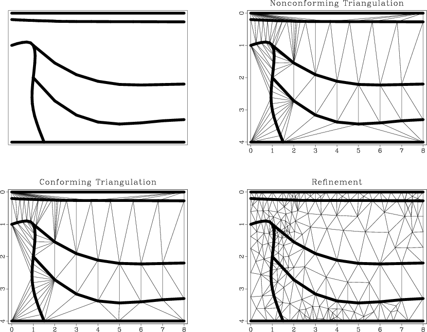
Figure H-9 demonstrates an application of different triangulation techniques to a simple layered model, borrowed from the Seismic Unix demos (where it is attributed it to V.Cervený.) Another model from Hale and Cohen (1991) is used in Figure H-10.

cerveny
Figure A-9. A comparison of different triangulation techniques on a simple layered model. The top left plot shows the original model; the top right plot, the result of noncomforming triangulation; the two bottom plots, conforming triangulation and an additional mesh refinement.

susalt
Figure A-10. A comparison of different triangulation techniques on a simple salt-type model. The top left plot shows the original model; the top right plot, the result of noncomforming triangulation; the two bottom plots, conforming triangulation and an additional two-step mesh refinement.

A variational formulation of the fast marching eikonal solver