A variational formulation of the fast marching eikonal solver

The theoretic grounds of variational principles

This section serves as a brief reminder of the well-known theoretical connection between Fermat's principle and the eikonal equation. The reader, familiar with this theory, can skip safely to the next section.

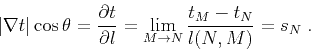
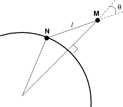
fermat Figure 2. Illustration of the connection between Fermat's principle and the eikonal equation. The shortest distance between a wavefront and a neighboring point $M$ is along the wavefront normal.

Both Fermat's principle and the eikonal equation can serve as the foundation of traveltime calculations. In fact, either one can be rigorously derived from the other. A simplified derivation of this fact is illustrated in Figure 2. Following the notation of this figure, let us consider a point $M$ in the immediate neighborhood of a wavefront $t (N) = t_N$. Assuming that the source is on the other side of the wavefront, we can express the traveltime at the point $M$ as the sum

$$t_M = t_N + l (N,M) s_M\;,$$ (3)

where $N$ is a point on the front, $l (N,M)$ is the length of the ray segment between $N$ and $M$, and $s_M$ is the local slowness. As follows directly from equation (3),

$$\left\vert\nabla t\right\vert \cos{\theta} = \frac{\partial... ...} = \lim_{M \rightarrow N} \frac{t_M - t_N}{l (N,M)} = s_N\;.$$ (4)

Here $\theta$ denotes the angle between the traveltime gradient (normal to the wavefront surface) and the line from $N$ to $M$, and $\frac{\partial t}{\partial l}$ is the directional traveltime derivative along that line.

If we accept the local Fermat's principle, which says that the ray from the source to $M$ corresponds to the minimum-arrival time, then, as we can see geometrically from Figure 2, the angle $\theta$ in formula (4) should be set to zero to achieve the minimum. This conclusion leads directly to the eikonal equation (2). On the other hand, if we start from the eikonal equation, then it also follows that $\theta=0$, which corresponds to the minimum traveltime and constitutes the local Fermat's principle. The idea of that simplified proof is taken from Lanczos (1966), though it has obviously appeared in many other publications. The situations in which the wavefront surface has a discontinuous normal (given raise to multiple-arrival traveltimes) require a more elaborate argument, but the above proof does work for first-arrival traveltimes and the corresponding viscosity solutions of the eikonal equation (Lions, 1982).

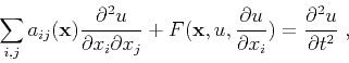
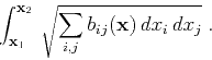
The connection between variational principles and first-order partial-differential equations has a very general meaning, explained by the classic Hamilton-Jacobi theory. One generalization of the eikonal equation is

$$\sum_{i,j} a_{ij} (\mathbf{x}) \frac{\partial \tau}{\partial x_i} \frac{\partial \tau}{\partial x_j} = 1\;,$$ (5)

where $\mathbf{x} = \{x_1, x_2, \ldots\}$ represents the vector of space coordinates, and the coefficients $a_{ij}$ form a positive-definite matrix $A$. Equation (5) defines the characteristic surfaces $t = \tau (\mathbf{x})$ for a linear hyperbolic second-order differential equation of the form

$$\sum_{i,j} a_{ij} (\mathbf{x}) \frac{\partial^2 u}{\partia... ...tial u}{\partial x_i}) = \frac{\partial^2 u}{\partial t^2}\;,$$ (6)

where F is an arbitrary function.

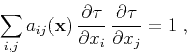
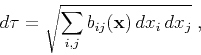
A known theorem (Smirnov, 1964) states that the propagation rays [characteristics of equation (5) and, correspondingly, bi-characteristics of equation (6)] are geodesic (extreme-length) curves in the Riemannian metric

$$d \tau = \sqrt{\sum_{i,j} b_{ij} (\mathbf{x}) dx_i dx_j}\;,$$ (7)

where $b_{ij}$ are the components of the matrix $B = A^{-1}$. This means that a ray path between two points $\mathbf{x}_1$ and $\mathbf{x}_2$ has to correspond to the extreme value of the curvilinear integral

$$\int_{\mathbf{x}_1}^{\mathbf{x}_2} \sqrt{\sum_{i,j} b_{ij} (\mathbf{x}) dx_i dx_j}\;.$$

For the isotropic eikonal equation (2), $a_{ij} = \delta_{ij}/s^2 (\mathbf{x})$, and metric (7) reduces to the familiar traveltime measure

$$d \tau = s (\mathbf{x}) d\sigma\;,$$ (8)

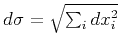where $d\sigma = \sqrt{\sum_{i} dx_i^2}$ is the usual Euclidean distance metric. In this case, the geodesic curves are exactly Fermat's extreme-time rays.

From equation (7), we see that Fermat's principle in the general variational formulation applies to a much wider class of situations if we interpret it with the help of non-Euclidean geometries.

A variational formulation of the fast marching eikonal solver