A variational formulation of the fast marching eikonal solver

Conforming Triangulation

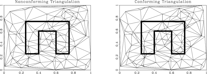
In the practice of mesh generation, the input nodes are often supplemented by boundary edges: geologic interfaces, seismic rays, and so on. It is often desirable to preserve the edges so that they appear as edges of the triangulation (Albertin and Wiggins, 1994). One possible approach is constrained triangulation, which preserves the edges, but only approximately satisfies the Delaunay criterion (Chew, 1989; Lee and Lin, 1986). An alternative, less investigated, approach is conforming triangulation, which preserves the ``Delaunayhood'' of the triangulation by adding additional nodes (Hansen and Levin, 1992) (Figure H-4). Conforming Delaunay triangulations are difficult to analyze because of the variable number of additional nodes. This problem was attacked by Edelsbrunner and Tan (1993), who suggested an algorithm with a defined upper bound on added points. Unfortunately, Edelsbrunner's algorithm is slow in practice because the number of added points is largely overestimated. I chose to implement a modification of the simple incremental algorithm of Hansen and Levin. Although Hansen's algorithm has only a heuristic justification and sets no upper bound on the number of inserted nodes, its simplicity is attractive for practical implementations, where it can be easily linked with the incremental algorithm of Delaunay triangulation.

The incremental solution to the problem of conforming triangulation can be described by the following scheme:

• First, the boundary nodes are triangulated.
• Boundary edges are inserted incrementally.
• If a boundary edge is not present in the triangulations, it is split in half, and the middle node is inserted into the triangulation. This operation is repeated for the two parts of the original boundary edge and continues recursively until all the edge parts conform.
• If at some point during the incremental process, a boundary edge violates the Delaunay criterion (the InCircle test), it is split to assure the conformity.

conform
Figure A-4. An illustration of conforming triangulation. The left plot shows a triangulation of 500 random points; the triangulation in the right plot is conforming to the embedded boundary. Conforming triangulation is a genuine Delaunay triangulation, created by adding additional nodes to the original distribution.

To insert an edge $AB$ into the current triangulation, I use the following recursive algorithm:

Function InsertEdge ($AB$)

1. Define $C$ to be the midpoint of $AB$.
2. Using the triangle tree structure, locate triangle $\mathcal{T} = DEF$ that contains $C$ in the current triangulation.
3. If $AB$ is an edge of $\mathcal{T}$ then return.
4. If $A$ (or $B$) is a vertex of $\mathcal{T}$ (for example, $A = D$) then define $C$ as an intersection of $AB$ and $EF$.
5. Else define $C$ as an intersection of $AB$ and an arbitrary edge of $\mathcal{T}$ (if such an intersection exists).
6. Insert $C$ into the triangulation.
7. InsertEdge ($CA$).
8. InsertEdge ($CB$).

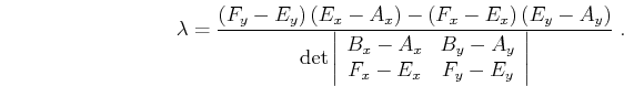
The intersection point of edges $AB$ and $EF$ is given by the formula

$$C = A + \lambda (B-A)\;,$$ (16)

where

$$\lambda = \frac{(F_y - E_y) (E_x - A_x) - (F_x - E_x) (E_... ...y - A_y \\ F_x - E_x & F_y - E_y \end{array}\right\vert}\;.$$ (17)

The value of $\lambda$ should range between $0$ and $1$.

If, at some stage of the incremental construction, a boundary edge $AB$ fails the Delaunay InCircle test for the circle $CABD$, then I simply split it into two edges by adding the point of intersection into the triangulation. The rest of the process is very much like the process of edge validation in the original incremental algorithm.

A variational formulation of the fast marching eikonal solver