|
|
|
|
Forward interpolation |
For completeness, I include a 2-D forward interpolation example. Figure 21 shows a 2-D analog of the function in Figure 4 and its coarsely-sampled version.

|
|---|
|
chirp2
Figure 21. Two-dimensional test function (left) and its coarsely sampled version (right). |
|
|
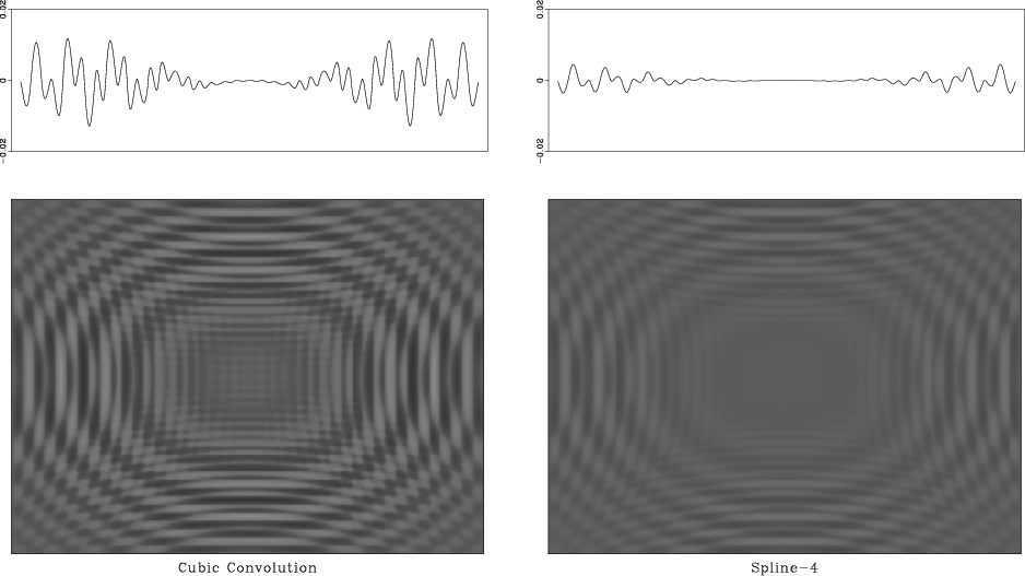
Figure 22 compares the errors of the 2-D nearest neighbor and 2-D linear (bi-linear) interpolation. Switching to bi-linear interpolation shows a significant improvement, but the error level is still relatively high. As shown in Figures 23 and 24, B-spline interpolation again outperforms other methods with comparable cost. In all cases, I constructed 2-D interpolants by orthogonal splitting. Although the splitting method reduces computational overhead, the main cost factor is the total interpolant size, which is squared when the interpolation goes from one to two dimensions.

|
|---|
|
plcbinlin
Figure 22. 2-D Interpolation errors of nearest neighbor interpolation (left) and linear interpolation (right). The top graphs show 1-D slices through the center of the image. Bi-linear interpolation exhibits smaller error and therefore is more accurate. |
|
|
|
|---|
|
plccubspl
Figure 23. 2-D Interpolation errors of cubic convolution interpolation (left) and third-order B-spline interpolation (right). The top graphs show 1-D slices through the center of the image. B-spline interpolation exhibits smaller error and therefore is more accurate. |
|
|

|
|---|
|
plckaispl
Figure 24. 2-D Interpolation errors of 8-point windowed sinc interpolation (left) and seventh-order B-spline interpolation (right). The top graphs show 1-D slices through the center of the images. B-spline interpolation exhibits smaller error and therefore is more accurate. |
|
|
|
|
|
|
Forward interpolation |