|
 |
 |
 | Theory of differential offset continuation |  |
![[pdf]](icons/pdf.png) |
Next: Example 1: plane reflector
Up: Introducing the offset continuation
Previous: Comparison with Bolondi's OC
To study the laws of traveltime curve transformation in the OC
process, it is convenient to apply the method of characteristics
(Courant, 1962) to the eikonal-type equation (4). The
characteristics of equation (4) [ bi-characteristics with respect to equation (1)]
are the trajectories of the high-frequency energy propagation in the
imaginary OC process. Following the formal analogy with seismic rays,
I call those trajectories time rays, where the word time
refers to the fact that the trajectories describe the traveltime
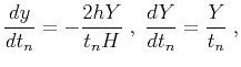
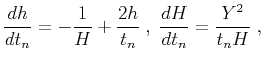
transformation (Fomel, 1994). According to the theory of first-order
partial differential equations, time rays are determined by a set of
ordinary differential equations (characteristic equations) derived
from equation (4) :
 |
|
|
|
 |
|
|
(23) |
where  corresponds to
 along a
ray and
along a
ray and  corresponds to
 . In this
notation, equation (4) takes the form
. In this
notation, equation (4) takes the form
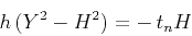 |
(24) |
and serves as an additional constraint for the definition of time
rays. System (23) can be solved by standard mathematical
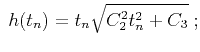
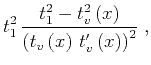
methods (Tenenbaum and Pollard, 1985). Its general solution takes the parametric form,
where the time variable  is the parameter changing along a time
ray:
is the parameter changing along a time
ray:
and  ,
,  , and
, and  are independent coefficients, constant
along each time ray. To find the values of these coefficients, we can
pose an initial-value problem for the system of differential
equations (23). The traveltime curve
are independent coefficients, constant
along each time ray. To find the values of these coefficients, we can
pose an initial-value problem for the system of differential
equations (23). The traveltime curve  for a
given common offset
for a
given common offset  and the first partial derivative
along the same constant offset section
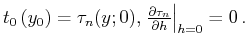
provide natural initial conditions. A particular case of those
conditions is the zero-offset traveltime curve. If the first partial
derivative of traveltime with respect to offset is continuous, it
vanishes at zero offset according to the reciprocity principle
(traveltime must be an even function of the offset):
and the first partial derivative
along the same constant offset section
provide natural initial conditions. A particular case of those
conditions is the zero-offset traveltime curve. If the first partial
derivative of traveltime with respect to offset is continuous, it
vanishes at zero offset according to the reciprocity principle
(traveltime must be an even function of the offset):
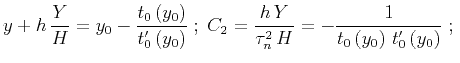
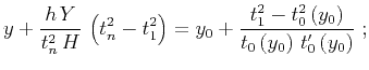
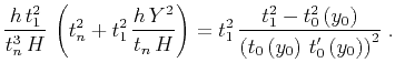
 Applying the initial-value conditions to the general
solution (26) generates the following expressions for the
ray invariants:
Applying the initial-value conditions to the general
solution (26) generates the following expressions for the
ray invariants:
where
 denotes the derivative
 . Finally, substituting
equations (27)
into (26), we obtain an explicit parametric form of the ray
trajectories:
. Finally, substituting
equations (27)
into (26), we obtain an explicit parametric form of the ray
trajectories:
Here  ,
,  , and
, and  are the coordinates of the continued
seismic section. Equations (28) indicates
that the time ray projections to a common-offset section have a
parabolic form. Time rays do not exist for
are the coordinates of the continued
seismic section. Equations (28) indicates
that the time ray projections to a common-offset section have a
parabolic form. Time rays do not exist for
 (a
locally horizontal reflector) because in this case post-NMO offset
continuation transform is not required.
(a
locally horizontal reflector) because in this case post-NMO offset
continuation transform is not required.
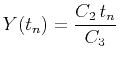
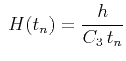
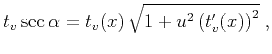
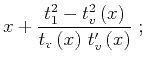
The actual parameter that
determines a particular time ray is the reflection point location.
This important conclusion follows from the known parametric equations
where  is the reflection point,
  is half of the wave velocity (
 ),
),
 is the vertical time (reflector depth divided by ), and
 is the
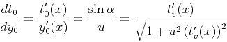
local reflector dip. Taking into account that the derivative of the zero-offset
traveltime curve is
is the
local reflector dip. Taking into account that the derivative of the zero-offset
traveltime curve is
 |
(32) |
and substituting equations (30) and (31)
into (28) and (29), we get
where
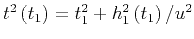 .
.
To visualize the concept of time rays, let us consider some simple
analytic examples of its application to geometric analysis of the
offset-continuation process.
Subsections
|
|
|
|
| Theory of differential offset continuation | |
|
Next: Example 1: plane reflector
Up: Introducing the offset continuation
Previous: Comparison with Bolondi's OC
2014-03-26