Seismic reflection data interpolation with differential offset and shot continuation

Offset continuation

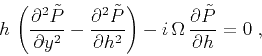
A particularly efficient implementation of offset continuation results from a log-stretch transform of the time coordinate (Bolondi et al., 1982), followed by a Fourier transform of the stretched time axis. After these transforms, the offset continuation equation from (Fomel, 2003) takes the form

$$h \, \left( {\partial^2 \tilde{P} \over \partial y^2} - {... ...i\,\Omega \, {\partial \tilde{P} \over {\partial h}} = 0 \;,$$ (1)

where $\Omega$ is the corresponding frequency, $h$ is the half-offset, $y$ is the midpoint, and $\tilde{P} (y,h,\Omega)$ is the transformed data. As in other $F$-$X$ methods, equation (1) can be applied independently and in parallel on different frequency slices.

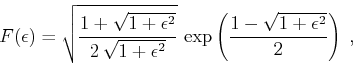
We can construct an effective offset-continuation finite-difference filter by studying first the problem of wave extrapolation between neighboring offsets. In the frequency-wavenumber domain, the extrapolation operator is defined by solving the initial-value problem on equation (1). The solution takes the following form (Fomel, 2003):

$$\widehat{\widehat{P}}(h_2) = \widehat{\widehat{P}}(h_1)\, Z_{\lambda}(kh_2)/Z_{\lambda}(kh_1)\;,$$ (2)

where $\lambda = (1 + i \Omega)/2$, and $Z_\lambda$ is the special function defined as

$$Z_{\lambda}(x) = \Gamma(1-\lambda)\,\left(x \over 2\right)^{\lambda}\, J_{-\lambda}(x)= {}_0F_1\left(;1-\lambda;-\frac{x^2}{4}\right)$$

$$= \sum_{n=0}^{\infty} {(-1)^n \over n!}\, {\Gamma(1-\lambda) \over \Gamma(n+1-\lambda)}\, \left(x \over 2\right)^{2n}\;,$$ (3)

where $\Gamma$ is the gamma function, $J_{-\lambda}$ is the Bessel function, and ${}_0F_1$ is the confluent hypergeometric limit function (Petkovsek et al., 1996). The wavenumber $k$ in equation (2) corresponds to the midpoint $y$ in the original data domain. In the high-frequency asymptotics, operator (2) takes the form

$$\widehat{\widehat{P}}(h_2) = \widehat{\widehat{P}}(h_1)\, F(... ...a\,\psi\left(2 k h_2/\Omega - 2 k h_1/\Omega\right)\right]}\;,$$ (4)

where

$$F(\epsilon)=\sqrt{{1+\sqrt{1+\epsilon^2}} \over {2\,\sqrt{1+... ...lon^2}}}\, \exp\left({1-\sqrt{1+\epsilon^2}} \over 2\right)\;,$$ (5)

and

$$\psi(\epsilon)={1 \over 2}\,\left(1 - \sqrt{1+\epsilon^2} + \ln\left({1 + \sqrt{1+\epsilon^2}} \over 2\right)\right)\;.$$ (6)

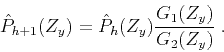
Returning to the original domain, we can approximate the continuation operator with a finite-difference filter with the $Z$-transform

$$\hat{P}_{h+1}(Z_y) = \hat{P}_{h} (Z_y) \frac{G_1(Z_y)}{G_2(Z_y)}\;.$$ (7)

The coefficients of the filters $G_1(Z_y)$ and $G_2(Z_y)$ are found by fitting the Taylor series coefficients of the filter response around the zero wavenumber. In the simplest case of 3-point filters, this procedure uses four Taylor series coefficients and leads to the following expressions:

$$G_1(Z_y) = 1 - \frac{1 - c_1(\Omega) h_2^2 + c_2(\Omega) h_1^2}{6} + \frac{1 - c_1(\Omega) h_2^2 + c_2(\Omega) h_1^2}{12}\, \left(Z_y + Z_y^{-1}\right)\;,$$ (8)

$$G_2(Z_y) = 1 - \frac{1 - c_1(\Omega) h_1^2 + c_2(\Omega) h_2^2}{6} + \frac{1 - c_1(\Omega) h_1^2 + c_2(\Omega) h_2^2}{12}\, \left(Z_y + Z_y^{-1}\right)\;,$$ (9)

where

$$c_1(\Omega) = \frac{3\,(\Omega^2 + 9 - 4 i\,\Omega)}{\Omega^2\,(3+i\,\Omega)}$$

and

$$c_2(\Omega) = \frac{3\,(\Omega^2 - 27 - 8 i\,\Omega)}{\Omega^2\,(3+i\,\Omega)}\;.$$

Figure 1 compares the phase characteristic of the finite-difference extrapolators (7) with the phase characteristics of the exact operator (2) and the asymptotic operator (4). The match between different phases is poor for very low frequencies (left plot in Figure 1) but sufficiently accurate for frequencies in the typical bandwidth of seismic data (right plot in Figure 1).

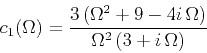
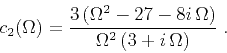
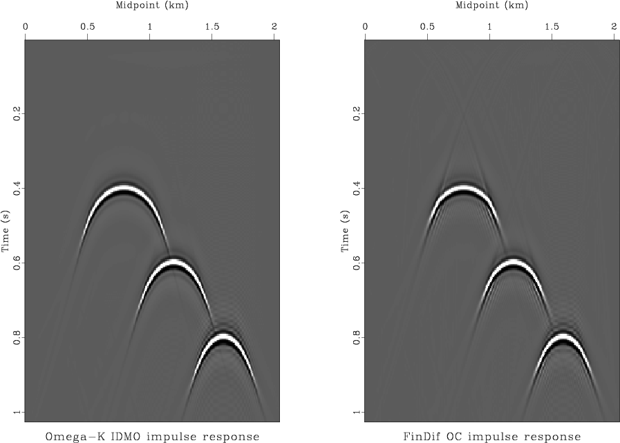
Figure 2 compares impulse responses of the inverse DMO operator constructed by the asymptotic $\Omega-k$ operator with those constructed by finite-difference offset continuation. Neglecting subtle phase inaccuracies at large dips, the two images look similar, which provides an experimental evidence of the accuracy of the proposed finite-difference scheme.

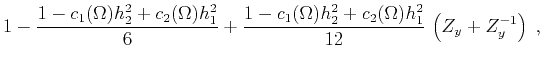
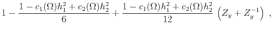
When applied on the offset-midpoint plane of an individual frequency slice, the one-dimensional implicit filter (7) transforms to a two-dimensional explicit filter with the 2-D $Z$-transform

$$G(Z_y,Z_h) = G_1(Z_y) - Z_h G_2(Z_y)\;.$$ (10)

Convolution with filter (10) is the regularization operator that I propose to use for interpolating prestack seismic data.

arg
Figure 1. Phase of the implicit offset-continuation operators in comparison with the exact solution. The offset increment is assumed to be equal to the midpoint spacing. The left plot corresponds to $\Omega =1$, the right plot to $\Omega =10$.

off-imp
Figure 2. Inverse DMO impulse responses computed by the Fourier method (left) and by finite-difference offset continuation (right). The offset is 1 km.

Seismic reflection data interpolation with differential offset and shot continuation