Applications of plane-wave destruction filters

High-order plane-wave destructors

Following the physical model of local plane waves, we can define the mathematical basis of the plane-wave destruction filters as the local plane differential equation

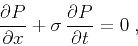$$\frac{\partial P}{\partial x} + \sigma\,\frac{\partial P}{\partial t} = 0\;,$$ (1)

where $P(t,x)$ is the wave field, and $\sigma$ is the local slope, which may also depend on $t$ and $x$. In the case of a constant slope, equation (1) has the simple general solution

$$P(t,x) = f(t - \sigma x)\;,$$ (2)

where $f(t)$ is an arbitrary waveform. Equation (2) is nothing more than a mathematical description of a plane wave.

If we assume that the slope $\sigma$ does not depend on $t$, we can transform equation (1) to the frequency domain, where it takes the form of the ordinary differential equation

$${\frac{d \hat{P}}{d x}} + i \omega\,\sigma\, \hat{P} = 0$$ (3)

and has the general solution

$$\hat{P} (x) = \hat{P} (0)\,e^{i \omega\,\sigma x}\;,$$ (4)

where $\hat{P}$ is the Fourier transform of $P$. The complex exponential term in equation (4) simply represents a shift of a $t$-trace according to the slope $\sigma$ and the trace separation $x$.

In the frequency domain, the operator for transforming the trace at position $x-1$ to the neighboring trace and at position $x$ is a multiplication by $e^{i \omega\,\sigma}$. In other words, a plane wave can be perfectly predicted by a two-term prediction-error filter in the $F$-$X$ domain:

$$a_0 \, \hat{P} (x) + a_1\, \hat{P} (x-1) = 0\;,$$ (5)

where $a_0 = 1$ and $a_1 = - e^{i \omega\,\sigma}$. The goal of predicting several plane waves can be accomplished by cascading several two-term filters. In fact, any $F$-$X$ prediction-error filter represented in the $Z$-transform notation as

$$A(Z_x) = 1 + a_1 Z_x + a_2 Z_x^2 + \cdots + a_N Z_x^N$$ (6)

can be factored into a product of two-term filters:

$$A(Z_x) = \left(1 - \frac{Z_x}{Z_1}\right)\left(1 - \frac{Z_x}{Z_2}\right) \cdots\left(1 - \frac{Z_x}{Z_N}\right)\;,$$ (7)

where $Z_1,Z_2,\ldots,Z_N$ are the zeroes of polynomial (6). According to equation (5), the phase of each zero corresponds to the slope of a local plane wave multiplied by the frequency. Zeroes that are not on the unit circle carry an additional amplitude gain not included in equation (3).

In order to incorporate time-varying slopes, we need to return to the time domain and look for an appropriate analog of the phase-shift operator (4) and the plane-prediction filter (5). An important property of plane-wave propagation across different traces is that the total energy of the propagating wave stays invariant throughout the process: the energy of the wave at one trace is completely transmitted to the next trace. This property is assured in the frequency-domain solution (4) by the fact that the spectrum of the complex exponential $e^{i \omega\,\sigma}$ is equal to one. In the time domain, we can reach an equivalent effect by using an all-pass digital filter. In the $Z$-transform notation, convolution with an all-pass filter takes the form

$$\hat{P}_{x+1}(Z_t) = \hat{P}_{x} (Z_t) \frac{B(Z_t)}{B(1/Z_t)}\;,$$ (8)

where $\hat{P}_x (Z_t)$ denotes the $Z$-transform of the corresponding trace, and the ratio $B(Z_t)/B(1/Z_t)$ is an all-pass digital filter approximating the time-shift operator  $e^{i \omega \sigma}$. In finite-difference terms, equation (8) represents an implicit finite-difference scheme for solving equation (1) with the initial conditions at a constant $x$. The coefficients of filter $B(Z_t)$ can be determined, for example, by fitting the filter frequency response at low frequencies to the response of the phase-shift operator. The Taylor series technique (equating the coefficients of the Taylor series expansion around zero frequency) yields the expression

$$B_3(Z_t) = \frac{(1-\sigma)(2-\sigma)}{12}\,Z_t^{-1} + ... ...sigma)(2-\sigma)}{6} + \frac{(1+\sigma)(2+\sigma)}{12}\,Z_t$$ (9)

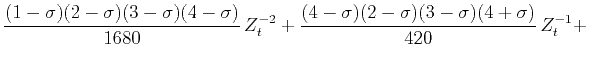
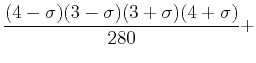
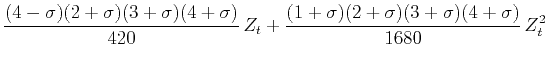
for a three-point centered filter $B_3(Z_t)$ and the expression

$$B_5(Z_t) = \frac{(1-\sigma)(2-\sigma)(3-\sigma)(4-\sigma)}{1680}\,Z_t^{-2} + \frac{(4-\sigma)(2-\sigma)(3-\sigma)(4+\sigma)}{420}\,Z_t^{-1} +$$

$$\frac{(4-\sigma)(3-\sigma)(3+\sigma)(4+\sigma)}{280} +$$

$$\frac{(4-\sigma)(2+\sigma)(3+\sigma)(4+\sigma)}{420}\,Z_t + \frac{(1+\sigma)(2+\sigma)(3+\sigma)(4+\sigma)}{1680}\,Z_t^2$$ (10)

for a five-point centered filter $B_5(Z_t)$. The derivation of equations (9-10) is detailed in the appendix. It is easy to generalize these equations to longer filters.

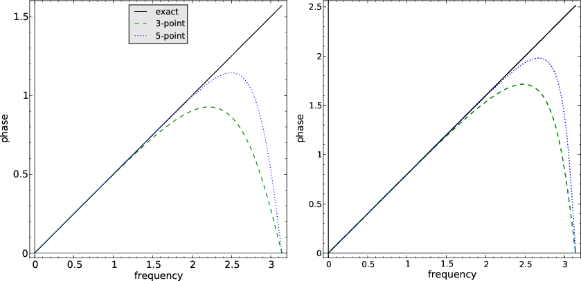
Figure 1 shows the phase of the all-pass filters $B_3(Z_t)/B_3(1/Z_t)$ and $B_5(Z_t)/B_5(1/Z_t)$ for two values of the slope $\sigma$ in comparison with the exact linear function of equation (4). As expected, the phases match the exact line at low frequencies, and the accuracy of the approximation increases with the length of the filter.

phase
Figure 1. Phase of the implicit finite-difference shift operators in comparison with the exact solution. The left plot corresponds to the slope of $\sigma =0.5$, the right plot to $\sigma =0.8$.

Taking both dimensions into consideration, equation (8) transforms to the prediction equation analogous to (5) with the 2-D prediction filter

$$A(Z_t,Z_x) = 1 - Z_x \frac{B(Z_t)}{B(1/Z_t)}\;.$$ (11)

In order to characterize several plane waves, we can cascade several filters of the form (11) in a manner similar to that of equation (7). In the examples of this paper, I use a modified version of the filter $A(Z_t,Z_x)$, namely the filter

$$C(Z_t,Z_x) = A(Z_t,Z_x) B(1/Z_t) = B(1/Z_t) - Z_x B(Z_t)\;,$$ (12)

which avoids the need for polynomial division. In case of the 3-point filter (9), the 2-D filter (12) has exactly six coefficients. It consists of two columns, each column having three coefficients and the second column being a reversed copy of the first one. When filter (12) is used in data regularization problems, it can occasionally cause undesired high-frequency oscillations in the solution, resulting from the near-Nyquist zeroes of the polynomial $B(Z_t)$. The oscillations are easily removed in practice with appropriate low-pass filtering.

In the next section, I address the problem of estimating the local slope $\sigma$ with filters of form (12). Estimating the slope is a necessary step for applying the finite-difference plane-wave filters on real data.

Applications of plane-wave destruction filters