Applications of plane-wave destruction filters

Signal and noise separation

Signal and noise separation and noise attenuation are yet another important application of plane-wave prediction filters. A random noise attention has been successfully addressed by Canales (1984), Gulunay (1986), Abma and Claerbout (1995), Soubaras (1995), and others. A more challenging problem of coherent noise attenuation has only recently joined the circle of the prediction technique applications (Guitton et al., 2001; Spitz, 1999; Brown and Clapp, 2000).

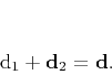
The problem has a very clear interpretation in terms of the local dip components. If two components, $\mathbf{s}_1$ and $\mathbf{s}_2$ are estimated from the data, and we can interpret the first component as signal, and the second component as noise, then the signal and noise separation problem reduces to solving the least-squares system

$$\mathbf{C}(\mathbf{s}_1) \mathbf{d}_1 \approx 0 \;,$$ (19)

$$\epsilon \mathbf{C}(\mathbf{s}_2) \mathbf{d}_2 \approx 0 \;$$ (20)

for the unknown signal and noise components $\mathbf{d}_1$ and $\mathbf{d}_2$ of the input data $\mathbf{d}$:

$$\mathbf{d}_1 + \mathbf{d}_2 = \mathbf{d}.$$ (21)

The scalar parameter $\epsilon$ in equation (20) reflects the signal to noise ratio. We can combine equations (19-20) and (21) in the explicit system for the noise component $\mathbf{d}_2$:

$$\mathbf{C}(\mathbf{s}_1) \mathbf{d}_2 \approx \mathbf{C}(\mathbf{s}_1) \mathbf{d}\;,$$ (22)

$$\epsilon \mathbf{C}(\mathbf{s}_2) \mathbf{d}_2 \approx 0\;.$$ (23)

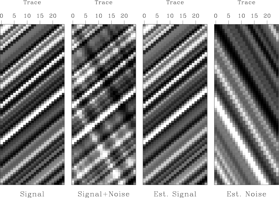
Figure 16 shows a simple example of the described approach. I estimated two dip components from the input synthetic data and separated the corresponding events by solving the least-squares system (22-23). The separation result is visually perfect.

sn2
Figure 16. Simple example of dip-based single and noise separation. From left to right: ideal signal, input data, estimated signal, estimated noise.

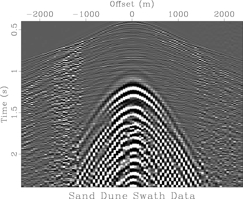
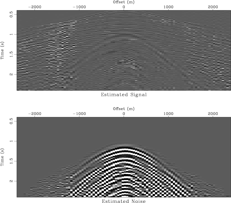
Figure 17 presents a significantly more complicated case: a receiver line from of a 3-D land shot gather from Saudi Arabia, contaminated with three-dimensional ground-roll, which appears hyperbolic in the cross-section. The same dataset has been used previously by Brown and Clapp (2000). The ground-roll noise and the reflection events have a significantly different frequency content, which might suggest separating them on the base of frequency alone. The result of frequency-based separation, shown in Figure 18 is, however, not ideal: part of the noise remains in the estimated signal after the separation. Changing the $\epsilon$ parameter in equation (23) could clean up the signal estimate, but it would also bring some of the signal into the subtracted noise. A better strategy is to separate the events by using both the difference in frequency and the difference in slope. For that purpose, I adopted the following algorithm:

1. Use a frequency-based separation (or, alternatively, a simple low-pass filtering) to obtain an initial estimate of the ground-roll noise.
2. Select a window around the initial noise. The further separation will happen only in that window.
3. Estimate the noise dip from the initial noise estimate.
4. Estimate the signal dip in the selected data window as the complimentary dip component to the already known noise dip.
5. Use the signal and noise dips together with the signal and noise frequencies to perform the final separation. This is achieved by cascading single-dip plane-wave destruction filters with local 1-D three-coefficient PEFs aimed at destroying a particular frequency.

The separation result is shown in Figure 19. The separation goal has been fully achieved: the estimated ground-roll noise is free of the signal components, and the estimated signal is free of the noise.

dune-dat
Figure 17. Ground-roll-contaminated data from Saudi Arabian sand dunes. A reciever cable out of a 3-D shot gather.

dune-exp
Figure 18. Signal and noise separation based on frequency. Top: estimated signal. Bottom: estimated noise.

dune-sn
Figure 19. Signal and noise separation based on both apparent dip and frequency in the considered receiver cable. Top: estimated signal. Bottom: estimated noise.

The examples in this subsection show that when the signal and noise components have distinctly different local slopes, we can successfully separate them with plane-wave destruction filters.

Applications of plane-wave destruction filters