|
 |
 |
 | Angle gathers in wave-equation imaging for transversely isotropic media |  |
![[pdf]](icons/pdf.png) |
Next: Numerical tests: The anisotropy
Up: Angle gathers in wave-equation
Previous: Introduction
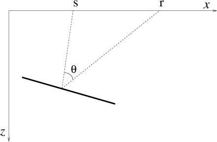
Relations between image coordinates and reflection (scattering) angles
at reflecting interfaces can be extracted by analyzing the geometry of
reflections in the simple case of a dipping reflector in a locally
homogeneous medium (Fomel, 2004). The geometry of the
reflection ray paths in 2-D is depicted in Figure 1(a).
|
|---|
raysr,rayparameters
Figure 1. (a) A schematic plot showing angle  . Although the model depicts a homogeneous setting, the
development will rely on the ray parameters defined in the immediate
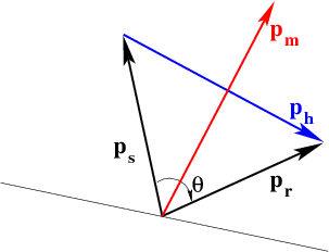
vicinity of the the reflection point, as shown in b.
(b) A schematic plot depicting the relation between the source and receiver ray-parameter vectors (
. Although the model depicts a homogeneous setting, the
development will rely on the ray parameters defined in the immediate
vicinity of the the reflection point, as shown in b.
(b) A schematic plot depicting the relation between the source and receiver ray-parameter vectors (
 and
and
 )
and the offset and midpoint vectors (
)
and the offset and midpoint vectors (
 and
and
 )
)
|
|---|
![[png]](icons/viewmag.png) ![[xfig]](icons/xfig.png)
|
|---|
According to elementary rules of geometry for the ray configuration in
Figures 1(a) and 1(b), with the
wavenumber vector given by
 as it relates to the
ray-parameter vector for a given angular frequency
as it relates to the
ray-parameter vector for a given angular frequency  , reflection 2opening (scattering)
phase angle
is represented by the following relation (Fomel, 2004; Sava and Fomel, 2005)
, reflection 2opening (scattering)
phase angle
is represented by the following relation (Fomel, 2004; Sava and Fomel, 2005)
 |
(1) |
where
 and
and
 are horizontal and vertical components of the offset
wave number, and
are horizontal and vertical components of the offset
wave number, and  and
and  are source and receiver wavenumber amplitudes related to their components as follows:
 ,
,
 ,
with
,
with
 ,
,
 ,
as suggested by Figure 1(b), where
,
as suggested by Figure 1(b), where
 is the horizontal component of the midpoint wavenumber.
To complete the system of equations necessary to relate angle
to midpoint and offset 2horizontal
wavenumbers, we use the dispersion
relation developed by Alkhalifah (1998) to define each of
 and
and
 as follows:
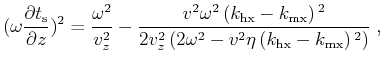
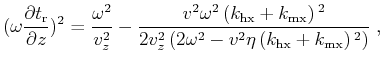
2where  is the NMO velocity. Using equation (1) in its expanded form and after some manipulation
and collecting terms with the same power of
is the NMO velocity. Using equation (1) in its expanded form and after some manipulation
and collecting terms with the same power of
 , we end up with the following quadratic equation:
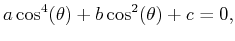 |
(4) |
with solutions given by
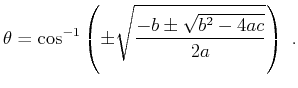 |
(5) |
Analytical representation of the coefficients is shown in
Table 1. The four solutions of
equation (5) are controlled by the sign of the offset
wavenumber and its magnitude compared with the midpoint wavenumber.
In the frequency-wavenumber domain, equation (5) can be
used to map offset 2(horizontal) wavenumbers to angle gathers for a specific
frequency, midpoint 2(horizontal) wavenumber, and depth slice. A description of an
algorithm to use with the mapping equation, in the case of an isotropic
medium, is given by Fomel (2004).
Setting  yields mapping for elliptical anisotropy with
coefficients of equation (5) given by
Table 2. The coefficients are represented by much
simpler formulas. In the isotropic case,
and
yields mapping for elliptical anisotropy with
coefficients of equation (5) given by
Table 2. The coefficients are represented by much
simpler formulas. In the isotropic case,
and  ,
Table 1 reduces to Table 3 and,
if substituted into the mapping formula of equation (5), is
equivalent to the corresponding mapping equation of
Fomel (2004).
,
Table 1 reduces to Table 3 and,
if substituted into the mapping formula of equation (5), is
equivalent to the corresponding mapping equation of
Fomel (2004).
|
|
|
|
| Angle gathers in wave-equation imaging for transversely isotropic media | |
|
Next: Numerical tests: The anisotropy
Up: Angle gathers in wave-equation
Previous: Introduction
2013-04-02