 |
 |
 |
 | Acoustic wavefield evolution as function of source location perturbation |  |
![[pdf]](icons/pdf.png) |
Next: The Green's function
Up: Alkhalifah: Source perturbation wave
Previous: Introduction
timedsS
Figure 2. Illustration of the relation between the initial source location and a perturbed version given by a single source and
image point locations. This is equivalent to a shift in the velocity field laterally by  . .
|

|
![[png]](icons/viewmag.png) ![[xfig]](icons/xfig.png)
|
|---|
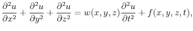
In this section, I derive partial differential equations that relate changes in the
wavefield shape to
perturbations in the source location. We will start by taking derivatives of the wave equation with respect
to lateral perturbation and then use the Taylor's series expansion to predict the wavefield form at another source.
In 3-D media, the acoustic wavefield  is described as a function of
  ,
,  and depth
  and is governed by a partial differential
equation as a function of time
and is governed by a partial differential
equation as a function of time  given by,
 |
|
|
(1) |
where  is the sloth (slowness squared) as a function position. and should be slowly varying with respect to the wavelength for proper
amplitude description. The source can be included as a function added to equation (1) 2given by
is the sloth (slowness squared) as a function position. and should be slowly varying with respect to the wavelength for proper
amplitude description. The source can be included as a function added to equation (1) 2given by  , defined usually at a point, or represented by the
wavefield
, defined usually at a point, or represented by the
wavefield  around time
  as an initial condition.
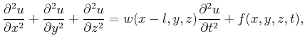
A change in the source location along the surface,2while keeping its source function stationary, is equivalently represented, in the far field,
by shifting the velocity field laterally
by the same amount in the opposite direction and thus can be represented by the following wave equation form:
as an initial condition.
A change in the source location along the surface,2while keeping its source function stationary, is equivalently represented, in the far field,
by shifting the velocity field laterally
by the same amount in the opposite direction and thus can be represented by the following wave equation form:
 |
|
|
(2) |
2where , in this case, is stationary and
independent of . A simple variable change of  can demonstrate this assertion, where
  is replaced by to
simplify notation. For simplicity, I use the symbol to describe the new wavefield, as well.
Figure 2 shows the depicts the relation for a single source and image point combination with the velocity shift.
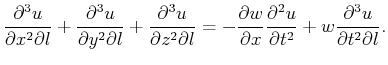
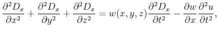
To evaluate the wavefield response to lateral perturbations,
we take the derivative of equation (2) with respect to , where the wavefield is
dependent on the source location as well [
is replaced by to
simplify notation. For simplicity, I use the symbol to describe the new wavefield, as well.
Figure 2 shows the depicts the relation for a single source and image point combination with the velocity shift.
To evaluate the wavefield response to lateral perturbations,
we take the derivative of equation (2) with respect to , where the wavefield is
dependent on the source location as well [ ], which yields:
 |
|
|
(3) |
Substituting
 , where is the equivalent source shift (actual velocity shift)
in the -direction, into equation (3), 2and setting
, where is the equivalent source shift (actual velocity shift)
in the -direction, into equation (3), 2and setting  , the location in which we evaluate the equation for the Taylor's series
expansion yields:
, the location in which we evaluate the equation for the Taylor's series
expansion yields:
 |
|
|
(4) |
which has the form of the wave equation with the last term on the right hand side acting as a source function. If this source function is zero given by, for example,
no lateral
velocity variation (
 =0), then
  =0, and as expected there will be no change in the wavefield form
with a change in source position.
=0, and as expected there will be no change in the wavefield form
with a change in source position.
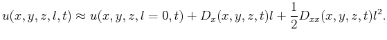
Therefore, the wavefield for a source located at a distance from the source used to estimate the wavefield can be approximated
using the following Taylor's series expansion:
 |
|
|
(5) |
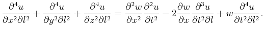
This result obviously has first-order accuracy represented by the first order Taylor's series expansion. For higher order accuracy, we take
the derivative of equation (3) again with respect to , which yields:
 |
|
|
(6) |
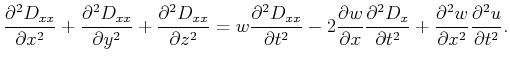
Again, by substituting
 , as well as, into equation (6) ,
2and setting , the
second order perturbation equation is given by:
, as well as, into equation (6) ,
2and setting , the
second order perturbation equation is given by:
 |
|
|
(7) |
Now, the wavefield for a source located at a distance from the original source can be approximated
using the following second-order Taylor's series expansion:
 |
|
|
(8) |
Equations (4) and (7) can be written in many forms and in the next section I show a velocity-derivative independent version of them.
2Equations (4) and (7) can be solved in many ways and in the next section I show some of the features gained by using an integral formulation given by the Green's function.
|
|
|
|
| Acoustic wavefield evolution as function of source location perturbation | |
|
Next: The Green's function
Up: Alkhalifah: Source perturbation wave
Previous: Introduction
2013-04-02