Least-squares diffraction imaging using shaping regularization by anisotropic smoothing

Workflow

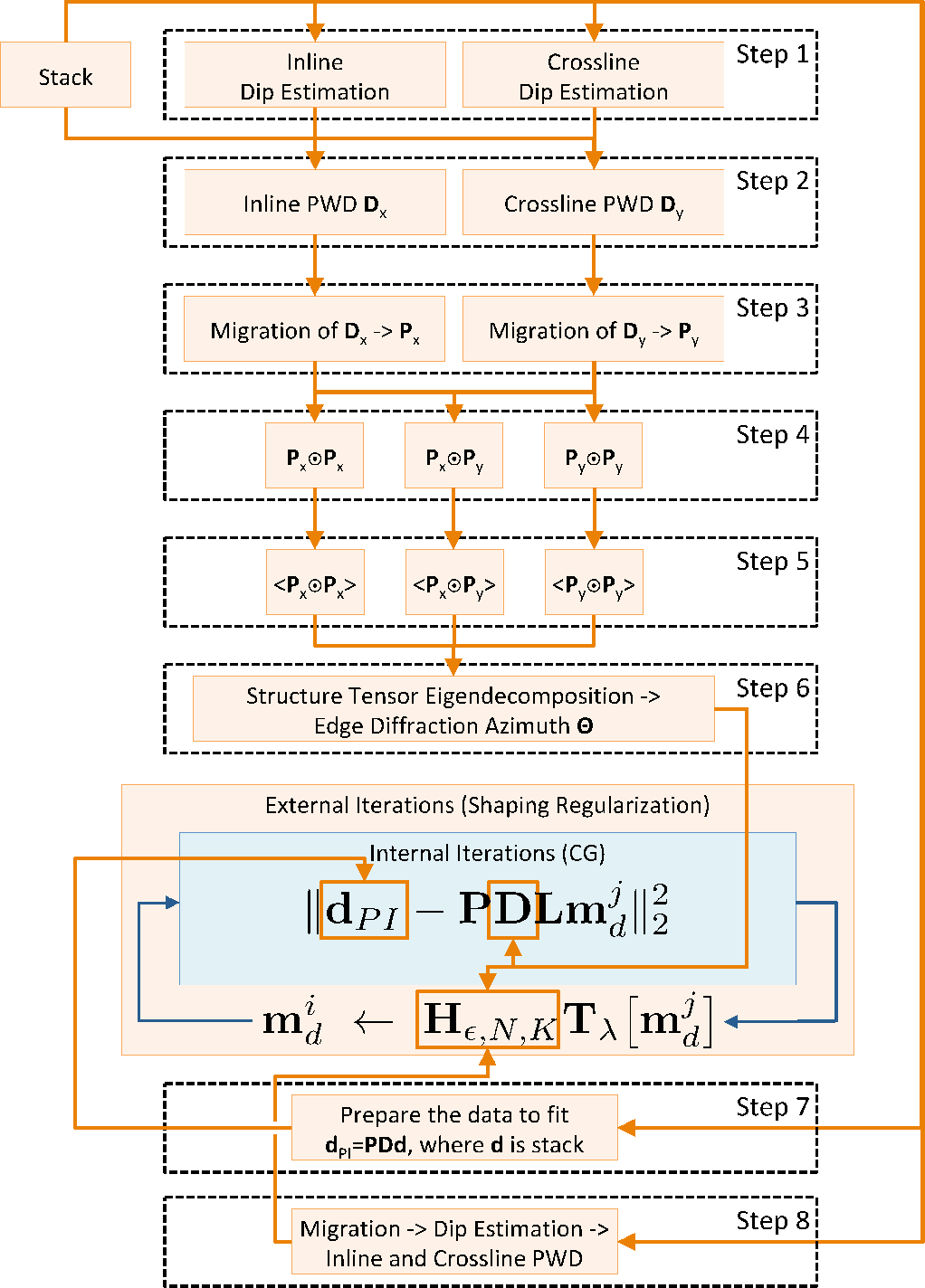
The workflow takes stacked data as the input. To generate all the inputs necessary for the inversion we propose the following sequence of procedures:

1. estimate inline and crossline dips describing dominant local slopes associated with reflections in the stack;
2. perform PWD filtering on the stack in inline and crossline directions;
3. migrate the corresponding volumes;
4. combine the migrated volumes in a structure tensor (equation 2);
5. smooth structure tensor components along structures with edge preservation;
6. perform eigendecomposition of a structure tensor and determine orientations of edges;
7. apply AzPWD and path-summation integral to the stacked data; apply conventional full-wavefield migration to the dataset stack (same as the input to step 1); estimate dips and generate PWD volumes in the inline and in the crossline directions in the image domain ( $\mathbf {D}_{\text {im}}$ in equation 3) for anisotropic smoothing regularization.

The sequence of procedures with their corresponding inputs and outputs is shown in Figure 2. In the first step, dips are estimated using PWD (Fomel et al., 2007), and two volumes - one for the inline dips and one for the crossline dips - are produced and further used for reflection removal in step 2. In the second step, based on the two input dip volumes, reflections are predicted and suppressed: two outputs are generated, which correspond to PWD filter application in the inline ( $\mathbf {D}_x$ ) and in the crossline ( $\mathbf {D}_y$ ) directions using the corresponding dip distributions. These two volumes with reflections removed are then migrated (step 3) using conventional full-wavefield migration, e.g. 3D post-stack Kirchhoff migration. For step 4, instead of explicitly computing structure tensor for each data sample according to equation 2, volumes for each of its components can be pre-computed. The term $p_x p_x$ structure-tensor component volume can be generated by the Hadamard product between the migrated inline PWD volume ( $\mathbf {P}_x$ ) and itself, the $p_y p_y$ -component volume - by the Hadamard product between the migrated crossline PWD volume ( $\mathbf {P}_y$ ) and itself, and the $p_x p_y$ -component volume - by the Hadamard product between the migrated inline PWD volume ( $\mathbf {P}_x$ ) and the migrated crossline PWD volume ( $\mathbf {P}_y$ ). Then, in step 5, the $p_x p_x$ , $p_y p_y$ , and $p_x p_y$ structure-tensor component volumes are input to edge preserving smoothing, which outputs the $\langle p_x p_x\rangle$ , $\langle p_y p_y\rangle$ , and $\langle p_y p_y\rangle$ volumes. In step 6, structure tensor (equation 2) eigendecomposition is performed ``on the fly'' by combining structure tensor component values from the $\langle p_x p_x\rangle$ , $\langle p_y p_y\rangle$ , and $\langle p_y p_y\rangle$ volumes for each data sample. The result is the smaller eigenvalue eigenvector volume, which is then converted to edge diffraction orientations $\mathbf {\Theta }$ . Step 7 gives the data to be fit by the inversion (equation 1). Orientations of structures for AzPWD and for anisotropic smoothing regularization are estimated in step 6. In anisotropic diffusion instead of derivatives in Cartesian coordinates we use PWDs in inline and crossline directions in the image domain ( $\mathbf {D}_{\text {im}}$ in equation 3), dip estimation for which should be performed on a ``conventional" image of a full wavefield stack (step 8). Then, we invert the data for edge diffractions.

schematic
Figure 2. Workflow chart illustrating the sequence of procedures and the relation of their corresponding inputs and outputs. Here, $\mathbf {D}_x$ and $\mathbf {D}_y$ correspond to inline and crossline PWD volumes of the input stack, $\mathbf {P}_x$ and $\mathbf {P}_y$ correspond to inline and crossline PWD volumes after migration, $\odot$ corresponds to the Hadamard (element-wise) matrix product, $\langle\rangle$ corresponds to the edge-preserved smoothing, $\mathbf {\Theta }$ corresponds to the volume of edge diffraction azimuths, $\mathbf {P}\mathbf {D}\mathbf {L}$ corresponds to the forward modeling operator corresponding to the chain of path-summation integral, AzPWD and Kirchhoff modeling operators respectively; $\mathbf {d}_{PI} = \mathbf {PDd}$ , where $\mathbf {d}$ corresponds to the input stack; and $\mathbf {H}_{\epsilon }$ and $\mathbf {T_{\lambda }}$ are anisotropic-smoothing and thresholding operators. The term $\mathbf {m}_d$ is the edge diffractivity we invert for: $\mathbf {m}_d^{j}$ describes model updates from internal iterations minimizing the misfit, and $\mathbf {m}_d^{i}$ is the result of regularization applied during external iterations. Notice in step 8, inline and crossline PWDs are computed in the image domain ( $\mathbf {D}_{\text {im}}$ in equation 3), and then are used instead of Cartesian derivatives in anisotropic smoothing operator $\mathbf {H}_{\epsilon }$ (equation 3). The edge diffraction azimuths $\mathbf {\Theta }$ are used in the AzPWD operator $\mathbf {D}$ (step 6) and in the anisotropic smoothing operator $\mathbf {H}_{\epsilon }$ to prevent smearing across the edges.

Least-squares diffraction imaging using shaping regularization by anisotropic smoothing