|
|
|
|
Non-hyperbolic common reflection surface |
|
|---|
|
dome,pick
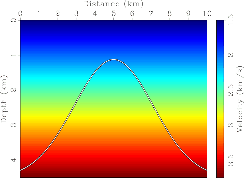
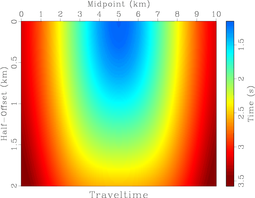
Figure 2. (a) Synthetic velocity model with a Gaussian-shape reflector. (b) Modeled reflection traveltime. |
|
|

|
|---|
|
crs-err4,ncrs-err4
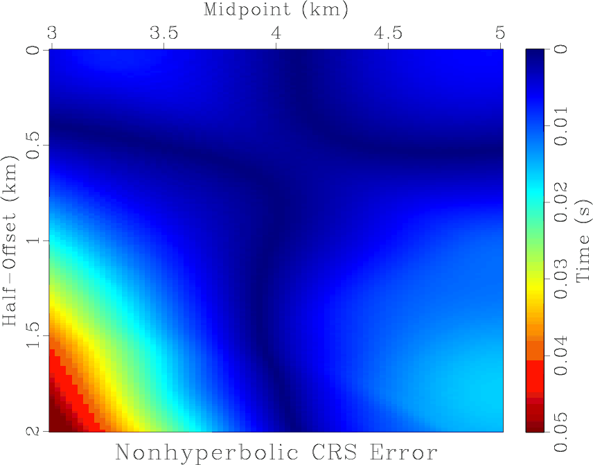
Figure 3. Absolute error of (a) CRS approximation, (b) nonhyperbolic CRS approximation. The reference midpoint is at 4 km. |
|
|
|
|---|
|
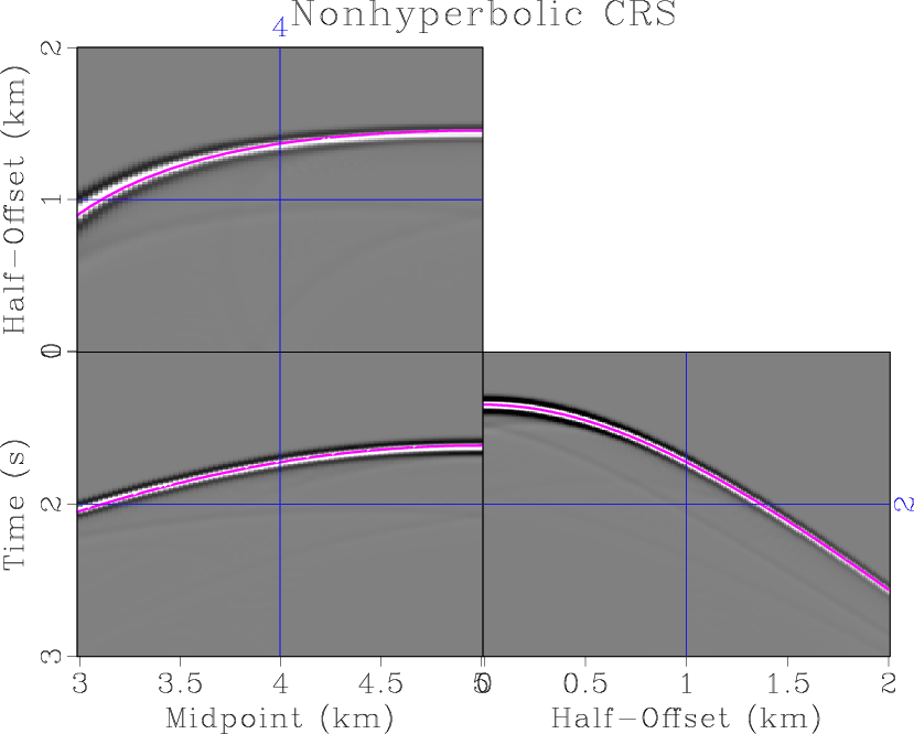
crs-data4,ncrs-data4
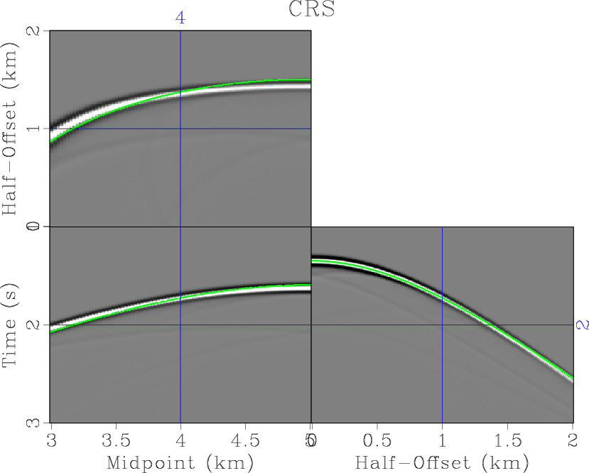
Figure 4. Modeled synthetic data with overlaid traveltime surfaces from least-squares fitting (colored curves). (a) CRS approximation. (b) Nonhyperbolic CRS approximation. The reference midpoint is at 4 km. |
|
|
In our next test, we generate a reflection traveltime surface by modeling reflection seismic data from a Gaussian-shape reflector, shown in Figure 2a by Kirchhoff modeling. The velocity changes linearly with depth. We extract the traveltime surface, shown in Figure 2b, and fit it with different approximations by non-linear least-squares optimization.
Our method for fitting the multivariate time-correction function
![]() (either CRS or nonhyperbolic
CRS) to a given experimental time data
(either CRS or nonhyperbolic
CRS) to a given experimental time data ![]() by finding optimal
parameters set
by finding optimal
parameters set
![]() is a minimization approach, defined as
follows:
is a minimization approach, defined as
follows:
The absolute error of CRS and nonhyperbolic CRS approximations, for a range of offsets and midpoints, is plotted in Figure 3. The nonhyperbolic CRS error is significantly smaller for a wide range of offsets and midpoints, which extends the applicability of the approximation. To effect of different approximations is shown additionally in Figure 4, which displays the modeled synthetic data with overlaid CRS and nonhyperbolic CRS approximations. The average relative error in different approximations, for the selected range of offsets and midpoints, is 1.24 % for the case of CRS and 0.41 % for the case of nonhyperbolic CRS. The average absolute error is 25 ms for the case of nonhyperbolic CRS and 8 ms for the case of nonhyperbolic CRS.
|
|
|
|
Non-hyperbolic common reflection surface |

![$\displaystyle \frac{\partial f}{\partial {a_i}} = \sum\limits_d\,\sum\limits_h ...
...0, \textbf{a}) - t(d,h) \right]\, \frac{\partial \hat{\theta}}{\partial a_i}\;.$](img59.png)