|
|
|
|
One-step slope estimation for dealiased seismic data reconstruction via iterative seislet thresholding |
Next: Conclusion Up: One-step slope estimation for Previous: Dealiased interpolation via one-step
|
|
|
|
One-step slope estimation for dealiased seismic data reconstruction via iterative seislet thresholding |
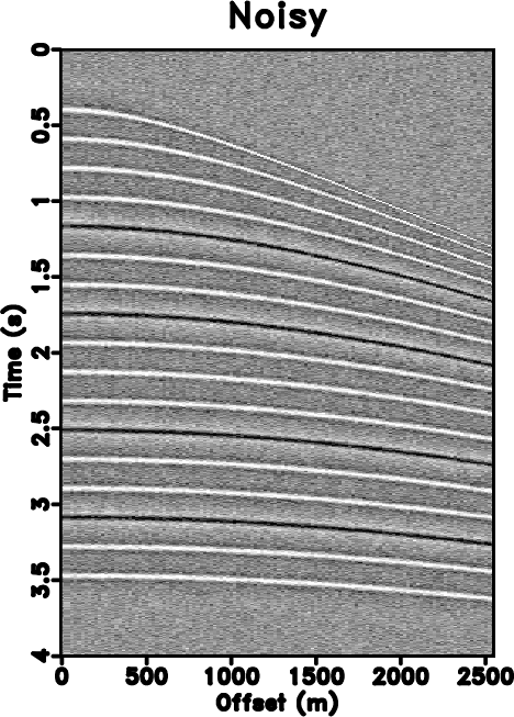
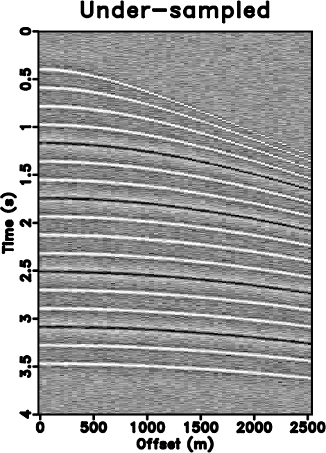
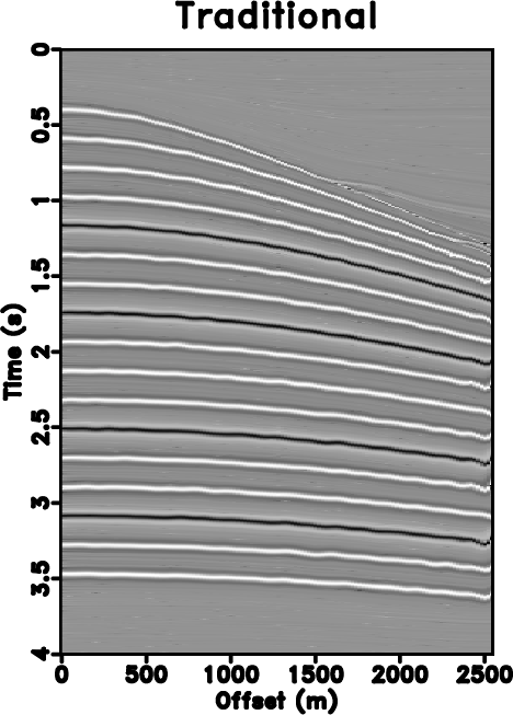
In order to test the influence of noise, we add some background noise to the synthetic example and conduct the same experiment as the clean data example. Figs. 5 and 6 show the reconstruction performance for the noisy data. Figs. 5a, 5b, and 5c show the noisy counterparts of Figs. 1a, 1b, and 1c. Figs. 5d, 5e, and 5f show the reconstructed results by using three different methods. Figs. 6a, 6b, and 6c show their corresponding error sections. In this noisy data experiment, the true model is still the clean data shown in Fig. 1a. By comparing the figures in Figs. 5 and 6, we can get a similar conclusion as the clean data experiment. The proposed approach can obtain the best performance, although the overall performance is worse than the clean data experiment. In this case, Spitz's method causes a lot of residual noise in the final result, since it is based on the prediction filter, which will inevitably predict the random noise.
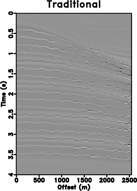
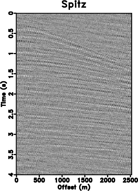
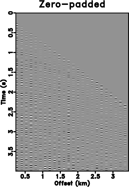
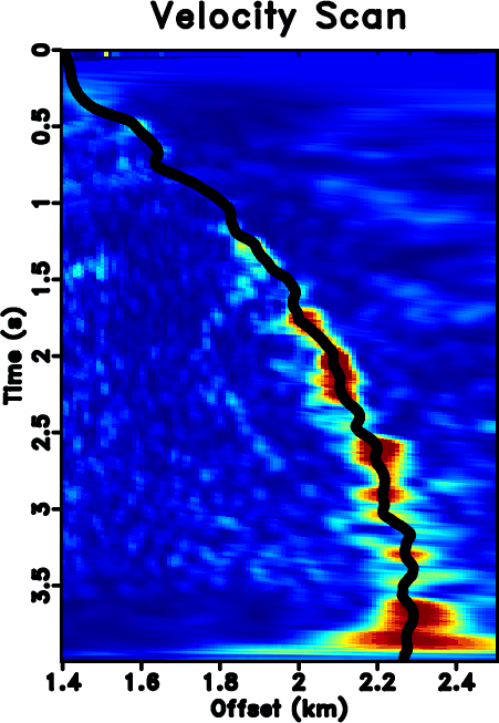
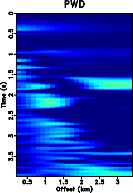
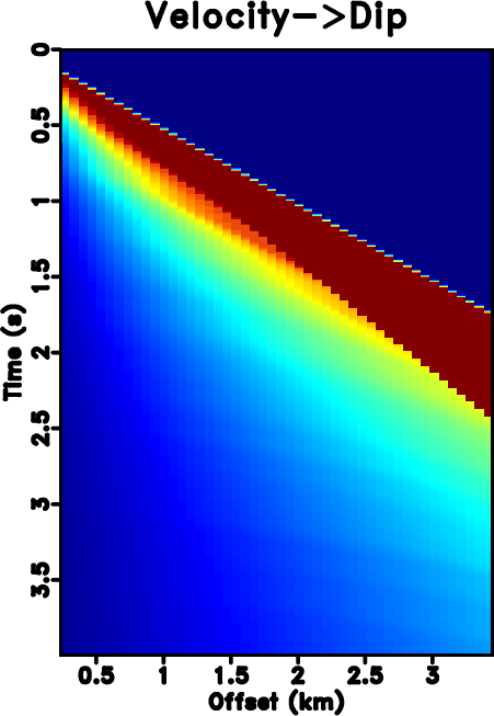
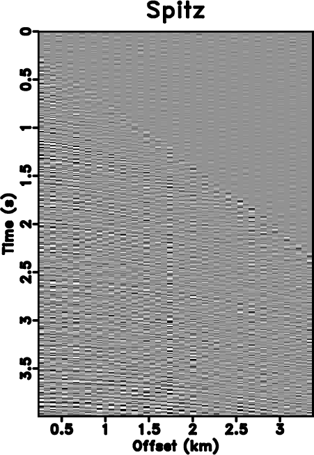
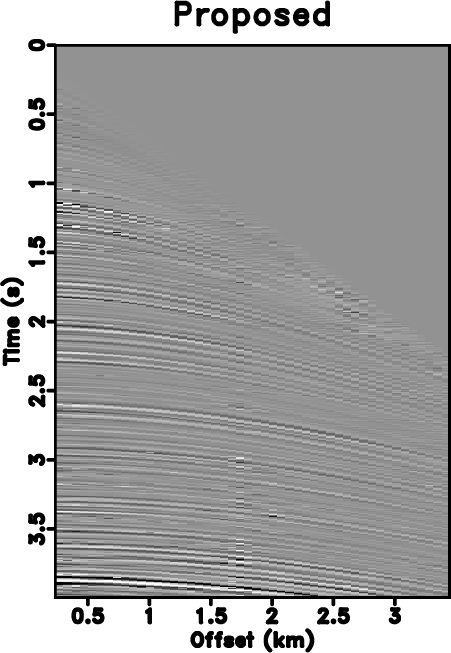
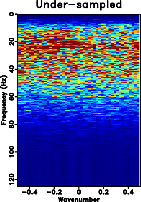
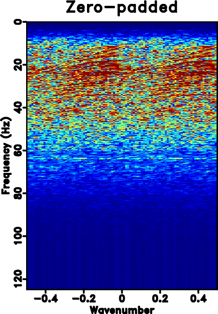
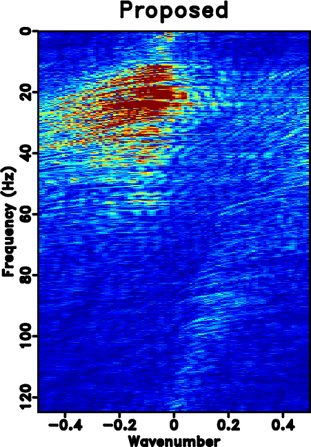
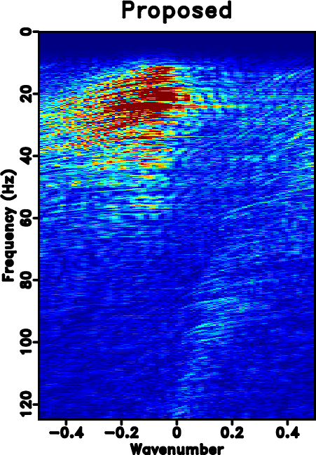
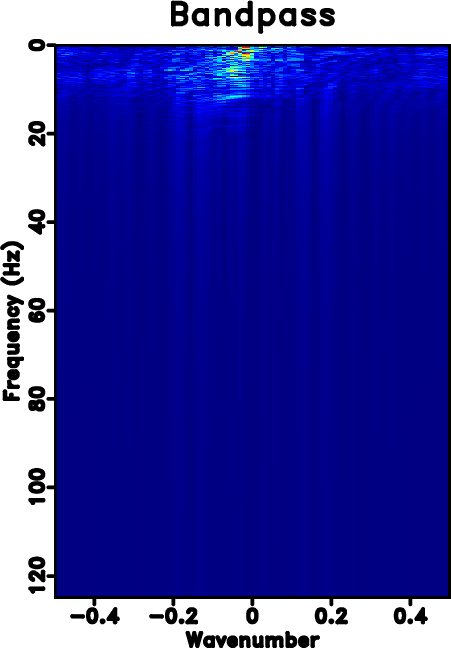
The next example is a poorly sampled marine dataset, which is shown in Fig. 7a. Fig. 7b shows the zero-padded data. Fig. 7c shows the NMO-based velocity analysis. The black string denotes the automatically picked NMO velocity. Fig. 7d shows the local slope calculated directly from the noisy and incomplete data by using the PWD algorithm (Fig. 7b). Fig. 7e shows the obtained local slope by using the velocity-slope transformation equation 4. The slope calculated through PWD algorithm is far from reasonable to capture the true local slope information of the data while the slope from the velocity-slope transformation can be interpreted well. Thus the latter method can be more stable in dealing with highly incomplete and noisy field datasets. Figs. 7f shows the result by using Spitz's method. Fig. 7g shows the result by using the proposed approach, which is of higher quality than Spitz's method. Figs. 8 shows the corresponding FK spectrum of different datasets, which also confirms that the aliasing problem is no longer existing after implementation of the proposed method. If observed carefully, some low-frequency low-wavenumber components can be discerned in Fig. 8d. In order to know exactly what these spectrum components represent in the time-space domain, we filter the final reconstructed result with a simple bandpass filter (with a bound frequency 9 Hz) and show the filtered result in Fig. 9a. Although we can not see obvious differences between Figs. 7g and 9a, we can find something in their difference section, as shown in Fig. 9b. The data shown on Fig. 9b corresponds to the low-frequency and low-wavenumber components of the field data, which is however very important to many seismic data processing tasks such as waveform inversion. Figs. 9c and 9d show the FK spectrum of Figs. 9a and 9b, respectively. Figs. 9c and 9d not only demonstrate the correctness of the bandpass filter, but also confirm the low-frequency data recovery property of the proposed algorithm.


|
|---|
|
hyper,hyper0,hyper-zero,hyper-seis,hyper-fx,hyper-seisvd
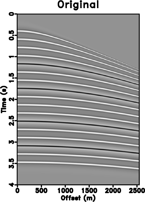
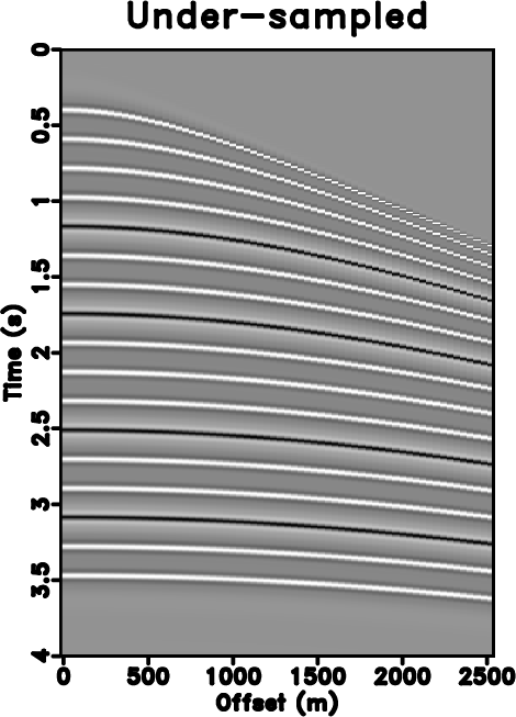
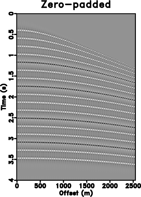
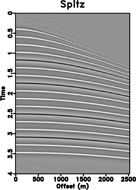
Figure 1. (a) Original synthetic data. (b) Under-sampled data. (c) Zero padded data (50% traces regularly removed). (d) Reconstructed data by using traditional iterative seislet thresholding. (e) Reconstructed data by using Spitz's method. (f) Reconstructed data by using the proposed approach. |
|
|
|
|---|
|
hyper-seis-dif,hyper-fx-dif,hyper-seisvd-dif
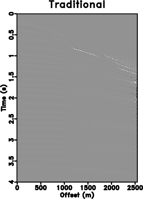
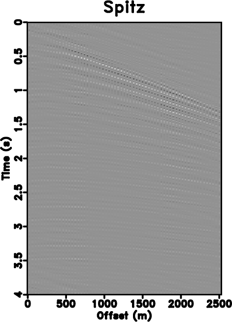
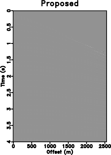
Figure 2. (a) Reconstruction error by using the traditional iterative seislet thresholding. (b) Reconstruction error by using Spitz's method. (c) Reconstruction error by using the proposed approach. |
|
|
|
|---|
|
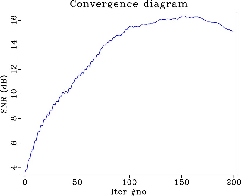
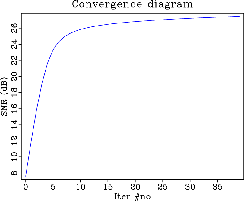
snrs-pocs,snrs-pocsvd
Figure 3. (a) SNRs by using the traditional iterative seislet thresholding. (b) SNRs by using the proposed approach. Please note that a large number of iterations can be saved and the performance can be improved. |
|
|

|
|---|
|
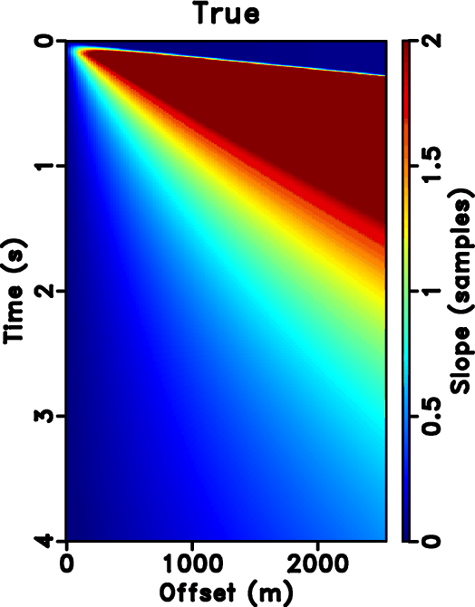
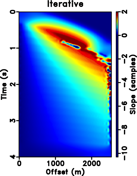
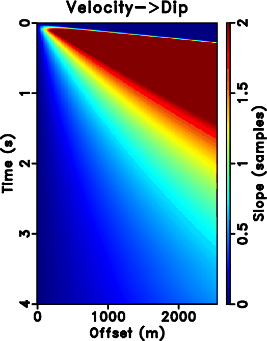
hyper-sdip,hyper-pdip,hyper-dipiter,hyper-vdip
Figure 4. (a) True slope. (b) Slope from PWD. (c) Slope estimated iteratively. (d) Slope from velocity-slope transformation. |
|
|


|
|---|
|
hyper-n,hyper0-n,hyper-zero-n,hypern-seis,hypern-fx,hypern-seisvd
Figure 5. (a) Noisy synthetic data. (b) Under-sampled data. (c) Zero padded data (50% traces regularly removed). (d) Reconstructed data by using traditional iterative seislet thresholding. (e) Reconstructed data by using Spitz's method. (f) Reconstructed data by using the proposed approach. |
|
|

|
|---|
|
hypern-seis-dif,hypern-fx-dif,hypern-seisvd-dif
Figure 6. Noisy data example. (a) Reconstruction error by using the traditional iterative seislet thresholding. (b) Reconstruction error by using Spitz's method. (c) Reconstruction error by using the proposed approach. |
|
|

|
|---|
|
bei,bei-zero,vscan,bei-pdip,bei-vdip,bei-fx,bei-seisvd
Figure 7. (a) Original under-sampled field data. (b) Zero padded data (with 50% traces regularly removed). (c) Velocity analysis result. (d) Local slope calculated directly from (b) by using the PWD algorithm. (e) Local slope calculated from the velocity-slope transformation. (f) Reconstructed data by using Spitz's method. (g) Reconstructed data by using the proposed approach. |
|
|

|
|---|
|
fk-bei,fk-bei-zero,fk-bei-fx,fk-bei-seisvd
Figure 8. FK spectrum of different sections. (a) Original under-sampled field data. (b) Zero padded data (with 50% traces regularly removed). (c) Reconstructed data by using Spitz's method. (d) Reconstructed data by using the proposed approach. |
|
|


|
|---|
|
bei-seis-bp,bei-dif-bp,fk-bei-seis-bp,fk-dif-bp
Figure 9. (a) Bandpass filtered result after iterative seislet thresholding with a bound frequency 9 Hz. (b) Low frequency data of the reconstructed data in Fig. 7g. (c) FK spectrum of (a). (d) FK spectrum of (b). |
|
|
|
|
|
|
One-step slope estimation for dealiased seismic data reconstruction via iterative seislet thresholding |