 |
 |
 |
 | Elastic wave-vector decomposition in heterogeneous anisotropic media |  |
![[pdf]](icons/pdf.png) |
Next: qS-wave polarization vectors in
Up: Review of wave-mode separation
Previous: Elastic wave-vector decomposition
For the wave-vector decomposition method, we focus on equation 14 and transform it to the space domain using the inverse Fourier transform as follows (Cheng and Fomel, 2014):
![$\displaystyle \mathbf{U}^{\alpha}\mathbf{(x)} = \int e^{i\mathbf{k}\cdot\mathbf...
...mathbf{x},\mathbf{\bar{k}})\mathbf{\widetilde{U}(\bar{k})}\right]d\mathbf{k} ~,$](img76.png) |
(15) |
where
 denotes the unseparated wavefield in the Fourier domain and
 denotes the decomposed wavefield of
 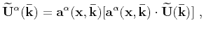 wave mode in the space domain. Equation 15 indicates that the unseparated wavefield is projected onto polarization vector
 of
wave mode in the Fourier domain and subsequently transformed back to the space domain for the final decomposed wavefield. The elements of matrix
of
wave mode in the Fourier domain and subsequently transformed back to the space domain for the final decomposed wavefield. The elements of matrix
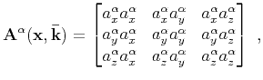 are given by
 |
(16) |
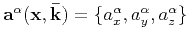
where
 and
and 
 and
and 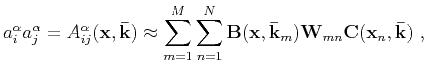 denoting different components.
Applying the low-rank approximation approach (Fomel et al., 2013), each element of
for a specified
wave mode in equation 15 and 16 can be approximated as follows (Cheng and Fomel, 2014):
 |
(17) |
where
 and
and
 are mixed-domain matrices with reduced wavenumber and spatial dimensions respectively;
 is a
is a  matrix with
 and
and  representing the rank of this low-rank decomposition.
One can view
representing the rank of this low-rank decomposition.
One can view
 as a submatrix of
 consisting of columns associated with
 , and
, and
 as a submatrix of
consisting of rows associated with
as a submatrix of
consisting of rows associated with
 . Physically, this process means that we only consider a selected few representative spatial locations (
 ) and representative wavenumbers (
 ), where
  is the size of the model, to build an effective approximation.
As a result, the low-rank approximation reduces computational cost by transforming the Fourier integral operator in equation 15 for each component
is the size of the model, to build an effective approximation.
As a result, the low-rank approximation reduces computational cost by transforming the Fourier integral operator in equation 15 for each component  and
and  denoting
 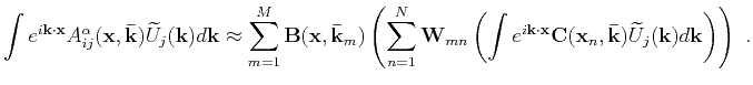 and
components to
and
components to
 |
(18) |
The computational cost of applying equation 18 is equivalent to the cost of
inverse fast Fourier Transforms (FFT) (Cheng and Fomel, 2014).
|
|
|
|
| Elastic wave-vector decomposition in heterogeneous anisotropic media | |
|
Next: qS-wave polarization vectors in
Up: Review of wave-mode separation
Previous: Elastic wave-vector decomposition
2017-04-18