Consider a block of 3D data
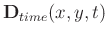 of
of  by
by  by
by  samples
 . The MSSA (Oropeza and Sacchi, 2011) operates on the data in the following way: first, MSSA transforms
into
. The MSSA (Oropeza and Sacchi, 2011) operates on the data in the following way: first, MSSA transforms
into
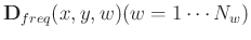 with complex values in the frequency domain. Each frequency slice of the data, at a given frequency
  , can be represented by the following matrix:
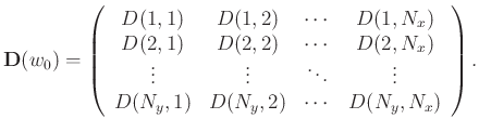 |
(1) |
To avoid notational clutter we omit the argument . Second, MSSA constructs a Hankel matrix for each row of
 ; the Hankel matrix
 for row
  of
is as follows:
of
is as follows:
 |
(2) |
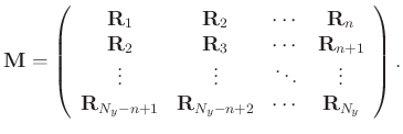
Then MSSA constructs a block Hankel matrix
 for
as:
for
as:
 |
(3) |
The size of
is  ,
,
 ,
,  .
.  and
and  are predifined integers chosen such that the Hankel maxtrix
and the block Hankel matrix
are close to square matrices, for example,
are predifined integers chosen such that the Hankel maxtrix
and the block Hankel matrix
are close to square matrices, for example,
 and
and
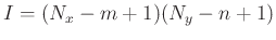
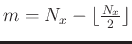
 , where
 denotes the integer part of the argument. We assume that
  . The filtered data are recovered with random noise attenuated by properly averaging along the anti-diagonals of the low-rank reduction matrix of
via TSVD. Next, we would like to briefly discuss the TSVD to introduce our work. In general, the matrix
can be represented as
. The filtered data are recovered with random noise attenuated by properly averaging along the anti-diagonals of the low-rank reduction matrix of
via TSVD. Next, we would like to briefly discuss the TSVD to introduce our work. In general, the matrix
can be represented as
 |
(4) |
where
 and
and
 denote the block Hankel matrix of signal and of random noise, respectively. We assume that
and
have full rank,
denote the block Hankel matrix of signal and of random noise, respectively. We assume that
and
have full rank,
 =
=
 and
has deficient rank,
and
has deficient rank,
 . The singular value decomposition (SVD) of
can be represented as:
. The singular value decomposition (SVD) of
can be represented as:
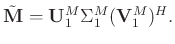
![$\displaystyle \mathbf{M} = [\mathbf{U}_1^M\quad \mathbf{U}_2^M]\left[\begin{arr...
...t[\begin{array}{c}
(\mathbf{V}_1^M)^H\\
(\mathbf{V}_2^M)^H
\end{array}\right],$](img47.png) |
(5) |
where
 (
( ) and
) and
 (
(
 ) are diagonal matrices and contain, respectively, larger singular values and smaller singular values.
 (
( ),
),
 (
(
 ),
),
 (
( ) and
) and
 (
(
 ) denote the associated matrices with singular vectors. The symbol
 ![$[\cdot]^H$](img60.png) denotes the conjugate transpose of a matrix. Generally, the signal is more energy-concentrated and correlative than the random noise. Thus, the larger singular values and their associated singular vectors represent the signal, while the smaller values and their associated singular vectors represent the random noise. We let
be
denotes the conjugate transpose of a matrix. Generally, the signal is more energy-concentrated and correlative than the random noise. Thus, the larger singular values and their associated singular vectors represent the signal, while the smaller values and their associated singular vectors represent the random noise. We let
be
 to achieve the goal of attenuating random noise as follows:
 |
(6) |
Equation 6 is referred to as the TSVD.
2020-02-21