|
|
|
|
Damped multichannel singular spectrum analysis for 3D random noise attenuation |
Next: Examples Up: Huang et al.: Damped Previous: Traditional MSSA by TSVD
|
|
|
|
Damped multichannel singular spectrum analysis for 3D random noise attenuation |
The singular value decomposition (SVD) of
![]() can be represented as:
can be represented as:
Because of the deficient rank, the matrix
![]() can be written as
can be written as
Combining equations 4, 7, and 8, we can factorize
![]() as follows:
as follows:
where ![]() and
and ![]() denote diagonal and positive definite matrices. Please note that M is constructed such that it is close to a square matrix (Oropeza and Sacchi, 2011), and thus the
denote diagonal and positive definite matrices. Please note that M is constructed such that it is close to a square matrix (Oropeza and Sacchi, 2011), and thus the ![]() and
and ![]() are assumed to be square matrices for derivation convenience. The appendix A provides the derivation of how we factorize
are assumed to be square matrices for derivation convenience. The appendix A provides the derivation of how we factorize
![]() into the form of equation 9. We observe that the left matrix has orthonormal columns and the middle matrix is diagonal. It can be proven that the right matrix also has orthonormal columns. The proof is provided in appendix A. Thus, equation 9 is an SVD of
into the form of equation 9. We observe that the left matrix has orthonormal columns and the middle matrix is diagonal. It can be proven that the right matrix also has orthonormal columns. The proof is provided in appendix A. Thus, equation 9 is an SVD of
![]() . According to the TSVD method, we let
. According to the TSVD method, we let ![]() be
be
![]() and then the following equation holds:
and then the following equation holds:
It is clear that
![]() . Because the matrices
. Because the matrices
![]() and
and
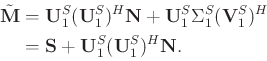
![]() are unknown, we cannot use equation 10 directly to attenuate the residual noise. However, by combining equations 6, 9 and 10, we can derive
are unknown, we cannot use equation 10 directly to attenuate the residual noise. However, by combining equations 6, 9 and 10, we can derive
![]() as:
as:
For simplification, we assume that there exist such
![]() and
and
![]() that
that
![]() and
and
![]() .
.
![]() is a square matrix of
is a square matrix of ![]() and
and
![]() is a diagonal matrix of
is a diagonal matrix of ![]() . Then we can simplify
. Then we can simplify
![]() as:
as:
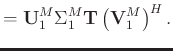
Inserting equations 14 and 15 into equation 13, we can obtain a simplified formula:
Combing equations 12 and 16, we can conclude that the true signal is a damped version of the previous TSVD method (equation 6), with the damping operator defined by equation 16. Right now, there is still one unknown parameter needed to be defined: ![]() . Although we have a potential selection
. Although we have a potential selection
![]() , as defined during the derivation of
, as defined during the derivation of
![]() , we cannot calculate it because we do not know
, we cannot calculate it because we do not know
![]() and
and
![]() .
.
Instead, we seek the form of ![]() from a different way. We treat
from a different way. We treat ![]() as a whole instead of paying attention to each detailed component in
as a whole instead of paying attention to each detailed component in
![]() . We have known that the true signal is a damped version of the TSVD method from the previous derivation, and the damping operator equals to
. We have known that the true signal is a damped version of the TSVD method from the previous derivation, and the damping operator equals to
![]() , acting on the diagonal matrix
, acting on the diagonal matrix
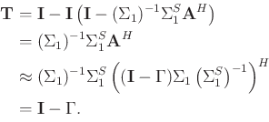
![]() . We can begin our search for an approximation of
. We can begin our search for an approximation of ![]() based on the following conditions:
based on the following conditions:
![\begin{displaymath}\Gamma=
\left(
\begin{array}{cccc}
a_1/b_1 & & & \\ [3mm]
& a...
...\ [3mm]
& & \ddots & \\ [3mm]
& & & a_K/b_K
\end{array}\right),\end{displaymath}](img95.png) |
(17) |
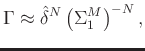
We tried a lot of numerical experiments and found that a very pleasant denoising performance can be obtained when ![]() is chosen as
is chosen as
Combining equations 12, 16, and 18, we conclude the approximation of
![]() as:
as:
The parameterization for the DMSSA approach is quite convenient. Although the traditional MSSA has a rank with broad range according to the data size and data complexity, the damping factor is usually chosen between 2-5. When damping factor is chosen as 1, the damping is very strong and will cause some useful energy loss, but when the damping factor is chosen as 2, 3, or even larger value, the compromise between preservation of useful signals and removal of random noise are much improved. The implementation of the DMSSA approach can be straightforwardly based on the MSSA framework, except for the slight difference, which introduces the damping factor.
|
|
|
|
Damped multichannel singular spectrum analysis for 3D random noise attenuation |
![$\displaystyle \mathbf{S} = [\mathbf{U}_1^S\quad \mathbf{U}_2^S]\left[\begin{arr...
...t[\begin{array}{c}
(\mathbf{V}_1^S)^H\\
(\mathbf{V}_2^S)^H
\end{array}\right].$](img64.png)
![$\displaystyle \mathbf{M} = [\mathbf{U}_1^S \quad \mathbf{U}_2^S]\left[\begin{ar...
...a_1^S)^H\\
(\Sigma_{2})^{-1}(\mathbf{N}^H\mathbf{U}_2^S)^H
\end{array}\right],$](img66.png)