|
|
|
|
First-break traveltime tomography with the double-square-root eikonal equation |
The first-break traveltime tomography with DSR eikonal equation (DSR tomography) can be established by following a procedure analogous to the traditional one with the shot-indexed eikonal equation (standard tomography). To further reveal their differences, in this section we will derive both approaches.
For convenience, we use slowness-squared
![]() instead of velocity
instead of velocity ![]() in equations 1,
3 and 4. Based on analysis in Appendix A, the velocity model
in equations 1,
3 and 4. Based on analysis in Appendix A, the velocity model ![]() and
prestack cube
and
prestack cube ![]() are Eulerian discretized and arranged as column vectors
are Eulerian discretized and arranged as column vectors ![]() of size
of size
![]() and
and ![]() of size
of size
![]() . We denote the observed first-breaks by
. We denote the observed first-breaks by
![]() , and use
, and use
![]() and
and
![]() whenever necessary to discriminate between
whenever necessary to discriminate between
![]() computed from shot-indexed eikonal equation and DSR eikonal equation.
computed from shot-indexed eikonal equation and DSR eikonal equation.
The tomographic inversion seeks to minimize the ![]() (least-squares) norm of the data residuals. We define
an objective function as follows:
(least-squares) norm of the data residuals. We define
an objective function as follows:
We start by deriving the Frechét derivative matrix of standard tomography. Denoting
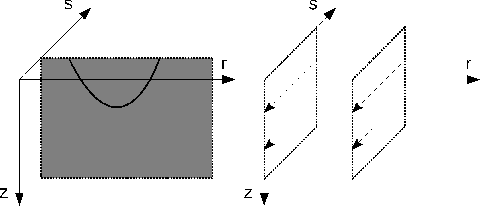
Figure 3 illustrates equation 12 schematically, i.e. the
gradient produced by standard tomography. The first step on the left depicts the transpose of the ![]() th Frechét
derivative acting on the corresponding
th Frechét
derivative acting on the corresponding ![]() th data residual. It implies a back-projection that takes
place in the
th data residual. It implies a back-projection that takes
place in the ![]() plane of a fixed
plane of a fixed ![]() position. The second step on the right is simply the summation
operation in equation 12.
position. The second step on the right is simply the summation
operation in equation 12.
|
|---|
|
cartonstd
Figure 3. The gradient produced by standard tomography. The solid curve indicates a shot-indexed characteristic. |
|
|
To derive the Frechét derivative matrix associated with DSR tomography, we first re-write equation
1 with definition 8
We recall that ![]() and
and ![]() are of different lengths. Meanwhile in equation 13, both
are of different lengths. Meanwhile in equation 13, both ![]() and
and ![]() have the size of
have the size of ![]() . Clearly in equation 14
. Clearly in equation 14
![]() and
and
![]() must achieve dimensionality enlargement.
In fact, according to Figure 1,
must achieve dimensionality enlargement.
In fact, according to Figure 1, ![]() and
and ![]() can be obtained by spraying
can be obtained by spraying ![]() such that
such that
![]() and
and
![]() . Therefore,
. Therefore,
![]() and
and
![]() are essentially spraying operators and their adjoints perform stackings along
are essentially spraying operators and their adjoints perform stackings along ![]() and
and
![]() dimensions, respectively.
dimensions, respectively.
In Appendix B, we prove that ![]() has the following form:
has the following form:
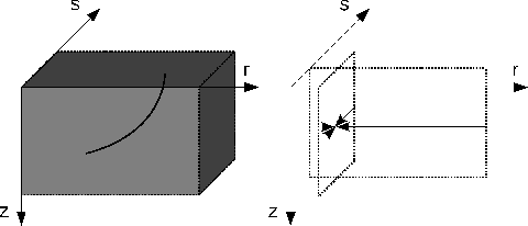
Figure 4 shows the gradient of DSR tomography. Similarly to the standard tomography, the
gradient produced by equation 16 is a result of two steps. The first step on the left is a
back-projection of prestack data residuals according to the adjoint of operator ![]() . Because
. Because ![]() contains
DSR characteristics that travel in prestack domain, this back-projection takes place in
contains
DSR characteristics that travel in prestack domain, this back-projection takes place in ![]() and is
different from that in standard tomography, although the data residuals are the same for both cases. The second
step on the right follows the adjoint of operators
and is
different from that in standard tomography, although the data residuals are the same for both cases. The second
step on the right follows the adjoint of operators ![]() and
and ![]() and reduces the dimensionality from
and reduces the dimensionality from ![]() to
to ![]() . However, compared to standard tomography this step involves summations in not only
. However, compared to standard tomography this step involves summations in not only ![]() but also
but also ![]() .
.
|
|---|
|
cartondsr
Figure 4. The gradient produced by DSR tomography. The solid curve indicates a DSR characteristic, which has one end in plane |
|
|
|
|
|
|
First-break traveltime tomography with the double-square-root eikonal equation |