Next: Preparing smoothly variable frequency
Up: Method
Previous: 1D non-stationary seislet transform
According to the autoregressive spectral analysis theory (Marple, 1987), a complex time series that has a constant frequency component is predictable by a two-point prediction-error filter
 . Suppose a complex time series is
  . In Z-transform notation, the two-point prediction-error filter can be expressed as:
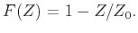 |
(13) |
We assume that a 1D time series has a smooth frequency component, then the 1D time series can be locally predicted using different local two-point prediction-error filters
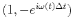 :
:
 |
(14) |
In order to estimate  using equation 14, we need to first minimize the least-squares misfit of the true and predicted time series with a local-smoothness constraint:
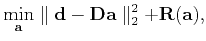 |
(15) |
where
 and
and
 are vectors composed of the entries
and
are vectors composed of the entries
and  , respectively, and
 .
.
 is a diagonal matrix composed of the entries
 .
.
 denotes the local-smoothness constraint. Equation 15 can be solved using shaping regularization:
![$\displaystyle \hat{\mathbf{a}} = [\lambda^2\mathbf{I}+\mathcal{T}(\mathbf{D}^T\mathbf{D}-\lambda^2\mathbf{I})]^{-1}\mathcal{T}\mathbf{D}^T\mathbf{d},$](img61.png) |
(16) |
where
 is a triangle smoothing operator and
  is a scaling parameter that controls the physical dimensionality and enables fast convergence.
can be chosen as the least-squares norm of
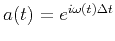
. After the filter coefficient
is obtained, we can straightforwardly calculate the local angular frequency
by
is a scaling parameter that controls the physical dimensionality and enables fast convergence.
can be chosen as the least-squares norm of
. After the filter coefficient
is obtained, we can straightforwardly calculate the local angular frequency
by
![$\displaystyle \omega(t) = Re\left[\frac{\mbox{arg}(a(t))}{\Delta t}\right].$](img64.png) |
(17) |
Next: Preparing smoothly variable frequency
Up: Method
Previous: 1D non-stationary seislet transform
2019-02-12